The content of this page has not been vetted since shifting away from MediaWiki. If you’d like to help, check out the how to help guide!
Introduction
Kymographs are a way to represent on a single image a dynamic process. They are particularly useful to monitor in a glimpse a moving organelle and characterize its motion. They can be seen as a x-t scan, where the intensity along a given line is plotted for all images of a stack. Each time point gives a intensity line, plotted e.g. along the x axis of the kymogrpah. These lines are stacked along the y axis for all frames. So we get an image where we move along space in the x direction and along time in the y direction.
Examples of usage can be found in the references listed at the end of this page. We will introduce them in a real-world example, using the most simple functions in ImageJ.
Context
This is a movie made in the lab of Ewa Paluch, MPI-CBG, featuring a floating L929 cell (mouse fibroblast), stained for myosin (RLC-GFP) being ablated in the cortex. The transmitted signal is overlayed with a confocal image of the GFP channel in various ways. The acto-myosin cortex is the part of the cytoskeletton that lies just below the membrane This cortex is active and generate a contractile force that presses on the cell volume. At rest, this tension gives the floating cell this spherical shape.
A picosecond pulsed laser allowed us to make a micro ablation of the cortex, without disrupting the membrane. The ablation laser power saturates the transmitted detector, which results in white frames in the movie.
When ablated at the left spot, the constraint on volume is relaxed, and the cortex can now contracts, expulsing some cytoplasm through the hole, like a relaxing ball that would be squeezed by your hands. This leads to the formation of a bleb, a woughly spherical bulge of membrane, initially devoid of cortex. After a while, a new cortex is polymerized and the bleb retracts. Goal of this study is to get the dynamics of the bleb growth and retraction.
Bleb growth dynamics
First, get the raw transmitted movie here (22MB).
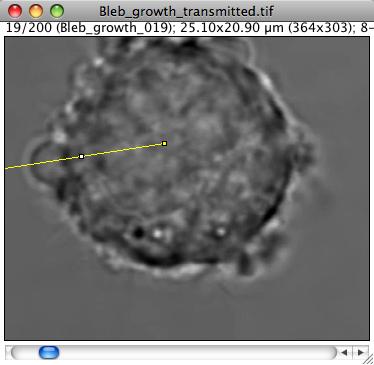
We would like to get the speed at which the front of the bleb grows. The simplest way to do so is to use kymographs. The idea is to draw a line from the center of the cell that passes through the bleb. To asjust the line position, select a frame where the bleb is still small, and draw a line ROI from the center through the bleb.
Check the feature using a profile plot (shortkey K or Analyze › Plot profile).
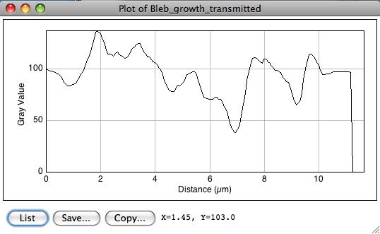
The edge feature is not that clear on this picture. At about 7 um, one can see that the dark pixels and the bright halo around the bleb front generated some kind of ridge.
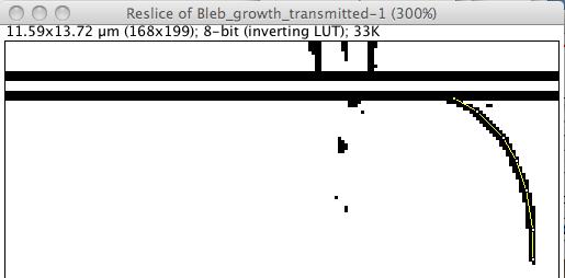
The kymograph consists in plotting this profile, encoding the intensity in grayscale level (or color for color images) for all slices. Rather than creating a plugin for this, we can use a function that was initially made for Z-stacks: the Image › Stacks › Reslice command (shortcut “/”). An option dialog appears; the defaults are fine for us, just press OK. We then get the kymograph:
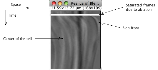
On this image, space is encoded along the x axis, following the line ROI from left to right. Since we drawn the ROI from the middle of the cell to the exterior of the cell, intensities measured within the cell are reported to the left of the image. At almost the extreme right, we get the cell’s border and the bleb front.
Time is encoded along the y direction. The first frame measurements is reported on the top line, and the bottom line reports the last frame. The white band correspond to the ablation, between frame 11 and 16, and appears between the 11 and 16 pixels of the kymograph.
ImageJ can’t deal with a calibration unit that is different in x and y axes, which is the case here (space and time). So for further analysis, we will have to put it right ourselves using the pixel size for the x calibration and the frame interval for the y calibration. I found it safer to remove totally any calibration from the images, even from the source stack. This way no confusion can be arise from a delay that would be measured in µm.
The front of the growing bleb can be seen below this white band, as a dark edge at the right of the image. The bleb growth appears here as a rather steep curve below the white band. Its retraction takes much longer, which results in having a drak edge slowly moving towards the left part of the image as we screoll down the kymograph. Other features within the cell can also be seen within its volume. In the case of this transmitted image, they are various granules movements which we do study here.
To get the bleb front dynamics, one can directly plot a multi- line ROI and get its coordinates for further analysis. We could also try to segment it a bit automatically.
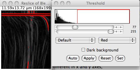
- Use the Process › Find edges command, to stress out the bleb front.
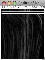
- Threshold it.
- Use the multi-line ROI to select points along the edge, and export their coordinates using the File › Save as… > XY Coordinates command.
You now have a text files made of 2 columns, the first one for the time, the second one for the bleb front position, ready for analysis. Do not forget to put the calibration right, tough.
Next step is to get numerical values and model for this growth. We leave it to another step, for the image analysis part is done.
Exercise: You can also think of a more clever way to extract the front coordinates, with sub-pixel accuracy (please share your ideas).
Myosin dynamics at bleb front
Now download here (22 MB) the movie for the same experiment, but measured in the fluorescence channel. It pictures myosin dynamics at the cortex. Our goal is to measure the myosin recovery rate at the bleb front during its growth. This would typically be complicated: we are trying to measure the intensity of something that moves over time. A sophisticated solution would be to segment the bleb front as an object and then measure the intensity given the objects. We propose here a simple solution involving a bit of manual interaction.
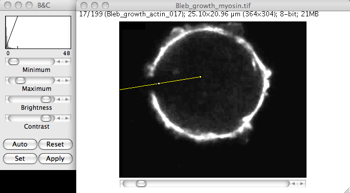
First,change a bit the contrast so that we can see the cortex well, so as to place correctly our line ROI. To do so, use Image › Adjust › Brightness/Contrast and play with the Maximum slider. Do not press Apply: we just want to improve what we see on the screen, not the actual intensities stored in the stack. Then draw a line ROI that goes - as before - from the center of the cell to the exterior, crossing the bleb grow spot.
Get the kymograph from this movie using the Reslice command. Thrash the calibration before doing it if you feel the use for it. You can also use the dynamic version of Reslice, shipped with Fijim and that can be found in Image › Stacks › Dynamic reslice. The advantage is that the kymograph is updated live when you move the ROI. After improving the contrast, it should look like this:
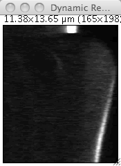
We can distinguish the bleb growth dynamics with this image, particularly on long delays when the acto-myosin cortex as repolymerized and reform a identifiable shell. It then appears at a bright band towards the bottom of the kymograph. We also have more or less our answer: along this bright band is pictured the myosin dynamics at the bleb front. To measure it across time, we just have to plot a profile that goes from the top of the kymograph to its bottom and that follows the bleb edge. The profile function has a nice features that allow to average over a certain line width. You can specify this width by double-clicking on the line tool button in the main Fiji window.
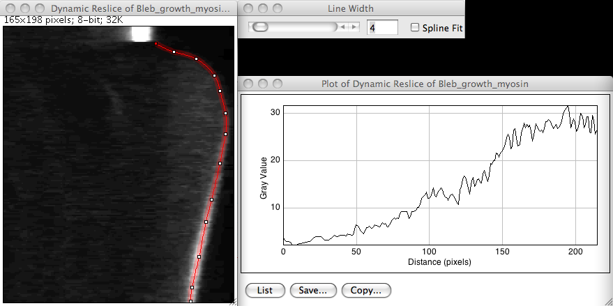
Plotting a profile on a kymograph
You can see that the myosin signal seems to recover very soon after ablation. But here is a gotcha that limits a bit the scope of this approach. Notice the units of the x axis of the profile. It is a distance in pixels where you expect a delay in seconds. It is anyway none of it, but an meaningless mix of both. The profile tool computes the distance that it reports in the x axis using the euclidian distance, that is
\[s=\sqrt{(x_2-x_1)^2+(y_2-y_1)^2}\]but since on our kymograph the x coordinates report the space and the y coordinates report the time, the x axis of the profile has no meaning, and can’t be exploited as is.
Exercise: Think of a way to put this right, that is to get a profile where the x axis would be the correct delay measured from the ablation offset (please discuss).