The page is a collection of principles for the entire image analysis process, from acquisition to processing to analysis.
Image acquisition
Introduction
Not all data is created equal and thus the analysis of certain images can be easily automated, while others pose a bigger challenge.
The goal of this section is to collect information on image acquisition principles that ease the automation of image analysis.
Use sufficient spatial resolution
Spatial resolution refers to the number (or density, if you prefer) of samples in the image. Digital detectors such as cameras and PMTs can produce sample matrices ranging from 256 x 256 pixels or fewer, up to 128 megapixels or more. As a rule of thumb, more samples is better. Spatial resolution can always be downsampled after the fact—but never upsampled. Furthermore, if your objects of interest are described by too few pixels, the error of many statistical computations will be prohibitively high, and some forms of analyses will not be possible at all.
Avoid lossy compression
Original data should be saved in a way that preserves the exact sample values. Do not store raw image data in file formats such as JPEG which use lossy compression. See Why (lossy) JPEGs should not be used in imaging below for details.
Illuminate as evenly as possible
Many forms of imaging require some form of illumination. You should ensure that this illumination is as evenly distributed as possible, rather than attempting to correct for it after acquisition. If you must tolerate an uneven illumination for some reason, try to acquire a background image so that you can use a background subtraction—but there may still be issues such as reflection artifacts.
Avoid overlapping objects
In many cases, it is not possible to avoid objects which overlap. But they are harder to analyze and measure, since many algorithms have difficulty distinguishing between objects. It may be possible to mitigate these difficulties by preparing the environment somehow—e.g., staining cell membranes with a fluorescent dye.
Naming schemes
Effective naming schemes are easy to read by both humans and computers. The following examples give an overview over the principles of creating good naming schemes:
- Example A:
Sample preparation
In certain cases (Examples …) it is very helpful to add markers to the slides.
Image analysis
Introduction
In scientific image processing and image analysis, an image is something different than a regular digital photograph of a beautiful scene you shot during your latest vacation.
In the context of science, digital images are samples of information, sampled at vertex points of n-dimensional grids.
What are pixel values?
Human visual perception is very good at certain tasks, such as contrast correction and detecting subtle differences in bright colors, but notoriously bad with other things, such as discerning dark colors, or classifying colors without appropriate reference. Our brains process and filter information, so that we perceive visually only after we 1) “see” light information that enters our eyes and interacts with the environment of the eye and eventually individual cells in our retinas, and 2) process the signal in the context of our brains. It is therefore very important to keep in mind that the pixel values in digital images are numbers, not subjective experiences of color. These numbers represent how light or some other type of signal entered the instrument we are using and interacted with its environment and eventually triggered sensors in the instrument that further processed the information into a digital output.
For example, when you record an image using a light gathering device such as a confocal microscope, the values you get at a certain coordinate or pixel are not color values, but relate to photon counts. This is an essential point to start with for understanding this topic.
Pixels are not little squares
And voxels are not cubes! See the whitepaper by Alvy Ray Smith.
Why (lossy) JPEGs should not be used in imaging
JPEG stands for Joint Photographic Experts Group who were the creators of a commonly used method of lossy compression for photographic images. This format is commonly used in web pages and supported by the vast majority of digital photographic cameras and image scanners because it can store images in relatively small files at the expense of image quality. There are also loss-less JPEG modes, but these in general are not widely implemented and chances are that most of the images are of the lossy type.
“Lossy compression” means that in the process of file size reduction certain amount of image information is discarded. In the case of JPEGs, this might not be readily obvious to an observer, but it will be important for image processing purposes.
“Loss-less or non-lossy compression” means that the file size is reduced, but the data stored is exactly the same as in the original.
In JPEG lossy compression, therefore, the stored image is not the same as the original, and hence not suitable for doing serious imaging work. While JPEG compression throws away information that the eye cannot detect easily, this results in considerable image artifacts (variable “blockiness” of the image in groups of 8x8 pixels). Any attempts to process or quantify those images will be affected in uncontrollable ways by the presence of the artifacts. This is particularly obvious in the hue channel of JPEG compressed colour images when converted to HSB colour space.
Example: a section of the famous Mandrill image. From left to right, you see the original (with an 8-bit colormap), the hue channel of the original, and the hue channel after saving as a JPEG with ImageJ’s default options – note in particular the vertical and horizontal artifacts:
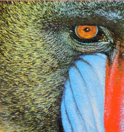
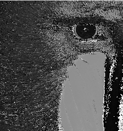
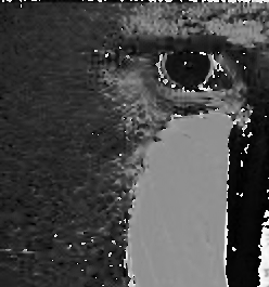
While most digital cameras save in JPEG format by default, it is very likely that they also support some non-lossy format (such as TIFF or a custom RAW format). Use those formats instead. A format called JPEG2000 supported by various slide scanners and used in “virtual slide” products was created to improve image quality and compression rates, however both lossy and non-lossy versions the JPEG2000 format exist. Use only the non-lossy formats.
Multichannel images in particular are harmed by the JPEG format: since the multiple channels are misinterpreted as red, green and blue (while most channels integrate more than just one wavelength), JPEG will shift the colors imperceptibly to improve compression. In the worst case, this can lead to colocalization where there was none.
TIFF or PNG formats available in ImageJ/Fiji are non-lossy formats. TIFF preserves any calibrations applied to your images, but images are not compressed. PNG files are smaller as non-lossy compression is applied but they do not store calibration data.
Once an image has been saved as compressed JPEG there is no way of reverting to the original, therefore an old JPEG-compressed image saved again as TIFF or PNG still contains all the original JPEG compression artifacts.
Below is an ImageJ macro which demonstrates the issue. It requires the Glasbey LUT, part of the Fiji distribution of ImageJ.
// load Boats
run("Boats (356K)");
run("Out [-]");
rename("Original");

// convert to JPEG
run("Duplicate...", " ");
run("Out [-]");
run("Save As JPEG... [j]", "jpeg=85");
run("Revert");
rename("JPEG");

// compute the difference
imageCalculator("Subtract create 32-bit", "Original","JPEG");
run("Out [-]");
rename("Difference");

// display windows side by side
run("Tile");

// highlight artifacts using Glasbey LUT
selectWindow("Original");
run("glasbey");
selectWindow("JPEG");
run("glasbey");
selectWindow("Difference");
Considerations during image segmentation (binarization)
What is binarization and what is it good for?
As the word already suggests, with a binarization you divide your image into two (not necessarily connected) parts usually referred to as foreground and background. This is the simplest method of image segmentation. “Simple” does not refer to easily achieving good results; it is, however, often perceived by the user as being easy to execute. There are also methods which group pixels of an image into different classes. Those ones are mostly based on statistical approaches. Some are implemented in Fiji such as the “Statistical Region Merging” plugin or the “Linear Kuwahara filter”. There exist even more sophisticated classification methods often based on machine learning and training by the user with a set of representative test images. While image binarization can also be achieved with methods including statistics the simplest would be to set one or two (upper and lower) cut-off value(s) separating specific pixel intensities from each other. This is often referred to as a threshold (value). Separating image features and objects by their intensity is often suitable if the intensity is the parameter which directly relates to the spatial characteristics of the objects and defines those. This is for example often the case in fluorescence microscopy with clearly stained cellular structures and low background staining. If other parameters define the structures outline or area, a simple threshold does often not lead to satisfying results or even fails completely doing the job. Many users are aware of a method which allows them to manually define such a threshold value but this comes with several limitations…
Why not simply choose a manual threshold?
“I usually define a manual threshold to extract my objects…, is this ok?” As a recommendation… Whenever possible, try to avoid manual thresholding!!!
Manual methods have several limitations:
- no/low reproducibility
- high user bias
- tedious and time-consuming fiddling-around finding an “appropriate” cut-off value
- incompatibility with automatic processing
- high intra- and inter-user variability
You might think of determining a fixed manual threshold and then applying the determined cut-off values to all your images. In this case, you face the decision of choosing one from 256 values. This would at least meet the criterion to treat equally all the images that you need to compare, but will not make you happy in the end. This is because there is a certain variability in the images of one single experiment and generally even higher variability between the images of replicated experiments, such that one fixed value will not extract similar features from different images. It is certainly a goal of digital image processing to establish protocols that eliminate variability, but currently a lofty goal, and even the most diligent of efforts to replicate circumstances generally fail to produce sets of images that can be thresholded with one fixed value. That is, it is not a realistic expectation in most fields.
So what is the alternative?
An alternative goal is to develop segmentation methods that overcome the variability. Indeed, segmentation algorithms have been a goal in biology and other areas for decades. The multifarious algorithms that have been developed are based on a vast array of different image properties (see below) but they all have in common that the determination of the threshold is based on image-intrinsic properties and not on subjective, real-time user decisions.
Inherently Subjective Components of Automated Segmentation
Being based on image-intrinsic properties does not mean automated segmentation methods are strictly objective and bias free. Obviously, since the user has a choice of algorithms, the final decision on which algorithm to apply under specific conditions or a specific experiment is necessarily subjective. This is itself a significant issue - for one thing, with respect to the decision posed earlier in this section about choosing from 256 possible cut-off values, the number of available algorithms is also high and continues to grow.
Moreover, an equally momentous problem is that segmentation methods are generally inherently biased in that they are trained in the first place against an initial human perception of what the final information extracted from an image should be. This is a reasonable basis of course, and its benefit is easily understood in the example of face recognition software trained to threshold faces based on human input on what constitutes a face. But the principle itself introduces bias. To understand negative consequences of this sort of bias, imagine a scenario in pathology, in which automated segmentation is developed to yield a certain result based on current expert pathologist experience, yet completely eliminates a cell feature that is later learned to be a critical indicator.
Automated segmentation is biased in other regards. Consider, for instance, the difference between global and local thresholds in binary segmentation. During global thresholding, the image as a whole is taken to determine the cut-off value and this value is applied to each pixel in the image. During local thresholding, in contrast, as the name suggests, values are determined in a local environment (often defined by the radius of a circular neighborhood) and the local cut-off values are locally applied to the individual pixels of the image. Thus, darker areas in an image might be extractable comparably as well as very bright areas, but this would not be possible with a global threshold, where specifically very dark areas shift into the background or might be under-extracted.
Benefits of Automated Segmentation
Their limitations notwithstanding, the advantages of automatic binarization methods are:
- they are fully reproducible (on the same image they will always lead to the same binarization result)
- they introduce no user bias during thresholding (this is not related to bias associated with the choice of specific automatic algorithm, which does exist)
- they use objectively determined cut-off values to minimize some variability in images being compared (e.g., algorithms that react to each image’s histogram often extract features deemed superior to features extracted using fixed values; but again, see the above note on a priori training of segmentation methods)
- they reduce preprocessing because they are easy applied to image stacks with variability between individual image histograms or in the complete stack histogram
- they are fast (no fiddling) and can be automated (e.g., in macros, plugins, batch jobs, etc.)
In ImageJ and Fiji, there are so far 16 Global Auto Thresholds and 9 Auto Local Thresholds implemented (by Gabriel Landini). These are very flexible and practical and can be integrated in macros and plugins, and do an excellent job for many intensity based images.
Is there one superior automatic algorithm?
For all of the reasons outlined above, NO! But this is not really a problem. It is akin to asking the question “Is there one superior food?”. As is the case with biological protocols in general, most algorithms are developed serving a specific purpose or solving a specific extraction problem. Thus, performance is relative and depends on the image content and quality, and the intended use of the pattern extracted. This last statement can be understood in terms of a single image from which an experimenter may want to extract overall cell shape in one investigation but nuclear texture in another. Every basic method needs to be tested to determine if any of its implementations do a good job for every single new question to be answered. In this regard, there are many more algorithms published and otherwise being developed, and you might want to think about implementing one in an ImageJ plugin yourself and providing it to the community :-)
Which automatic methods do exist for binarization?
Generally, there are different groups of algorithms for image binarization. (The following classification of methods is taken from Sezgin and Sankur, Survey over image thresholding techniques and quantitative performance evaluation, Journal of Electronic Imaging 13(1), 146–165 (January 2004).)
- Histogram shape-based methods, where, for example, the peaks, valleys and curvatures of the smoothed histogram are analyzed.
- Clustering-based methods, where the gray-level samples are clustered in two parts as background and foreground (object), or alternately are modelled as a mixture of two Gaussians.
- Entropy-based methods result in algorithms that use the entropy of the foreground and background regions, the cross-entropy between the original and binarized image, etc.
- Object attribute-based methods search a measure of similarity between the gray-level and the binarized images, such as fuzzy shape similarity, edge coincidence, etc.
- The spatial methods use higher-order probability distribution and/or correlation between pixels
- Local methods adapt the threshold value on each pixel to the local image characteristics.
This list might not be comprehensive but gives a good idea about the extensive possibilities available.
What else is critical during binarization and further object analysis?
Image acquisition
It is indispensable that during imaging the field of view be equally lit, and that this is checked and adjusted if necessary. Besides other disadvantages (e.g., no reliable intensity measurements), unequal lighting profoundly influences the outcome of thresholding methods, especially global ones. Furthermore, a higher signal-to-noise ratio, in e.g., fluorescence based images, will positively influence extraction by thresholding.
Pre-processing
Since the basis of any cut-off value during thresholding is pixel values, any change in those after image acquisition will also influence the final binarization result. Thus, the user needs to apply wisely methods that adjust brightness and contrast or any image filters, to not degrade but instead enhance the features of interest, fostering the binarization process. It may not be feasible to apply the same process to all images. In general, all pre-processing should be quantitated and recorded to ensure work is reproducible.
Post-processing
After being binarized through any thresholding method, an image may require additional binary operations to make the final pattern useable. These include erosion, dilation, opening, and closing (all under Process › Binary), image filters (under Process › Filters), and image combinations by boolean operations (e.g. Process › Image Calculator). Here the user needs to pay attention to recording all parameters and events and not alter the extraction notably, lest they reduce the reproducibility and overall quality of the segmentation. Post-processing binary operations might be necessary to correct further measurements of area or object counts. Internal holes, for example, may need to be closed (Process › Binary › Fill Holes) to extract the correct area of particles (this can also be achieved directly during the measurement when using >Analyze › Analyze Particles….). Watershed (or related) separation techniques may be necessary when close particles fuse to form clumps or aggregates.
Segmented ROIs for additional processing
Once an object is binarized, it can be converted to an ROI automatically and the ROI reapplied to the original image for verification as well as processing of the original image based on the ROI. This is used, for instance, to identify, separate, and analyze features of overlapping cells. The method for creating the ROIs from a binary image is Edit › Selection › Create Selection. This method is very useful when used with the RoiManager and in macros or plugins for automating tasks.
How do I check the quality of a binarization?
Several publications deal with methods to check the quality of image segmentation. Many methods refer to a comparison to a so called “ground truth” in the first place. For a user doing a binary segmentation, this is basically a user-created binarization of an example image to test the extraction “quality”. Similarly, when a method is being developed, benchmark images are created in a variety of ways including by taking photos of idealized objects and manually thresholding or tracing overlays to produce a desirable result or by generating computer simulations to form the standard against which the process will be assessed. Depending on the method, the original structures could include a range from simple forms to complex biological or synthetic structures of all sizes and shapes. Ideally, independent comparisons to different image-intrinsic measures (e.g., object edges, known angles or ratios between structural components, numbers of particular structural components, exclusion of known artifacts, entropy, etc.) should also be included when verifying the quality of a binarization. Of course, even for a simple round ball, this whole process has to be seen critically, because the accuracy of the result is necessarily defined by a biased “ground truth” in part defined by what the desired features to be extracted are. Thus, a researcher generally provides some degree of verification, explains its rationale, and acknowledges its limitations when commenting on the quality of a binarization.
A related issue is training the user. The “Threshold Check”, 1 is a trial to make it easier for the untrained user, to decide for one or the other threshold. The semi-quantitative evaluation therein is also biased but might facilitate a rather unbiased comparison of different extraction methods (based on a user-chosen and thus biased reference value).
What should I do with true color images (e.g. histological staining) with different colors and not a single intensity scale?
If converting to grayscale damages or distorts the information desired from a pattern, many different possibilities exist:
- One option, related to the manual thresholding methods mentioned above, is not ideal but has particular uses. It can be combined partially with automatic intensity thresholding and is mentioned here out of completeness since it might lead to good results (e.g., for some histological staining). The “Color Threshold” also implemented by Gabriel Landini gives access to different color space representations of a true color image. This means that the user can select specific ranges of color tones (hue) and color saturation as well as their brightness (e.g., using the HSB color space). In this case, a limitation to specific color tones using the hue value slider is possible with a rather low bias (if I want only blue, I exclude all the other colors, which is easier to determine than an intensity cut-off value). Saturation is already more tricky to set with low-subjectiveness. For the thresholding of the brightness, the standard Auto Thresholds can be applied, thus reducing the bias slightly.
- Similar to the method described above but more replicable, the image can be split into the respective channels of different color spaces (HSB, CIELAB,…) and those channels can then be automatically thresholded since all of them are based on a single intensity scale. It might already be sufficient to extract the desired information by thresholding only one of the color space channels. A combination of the extraction results from two or all three channels is also possible by using boolean functions (such as AND, OR, XOR) where applicable. This method is very effective with the right images (e.g., it can identify and separate overlapping cells).
- Color deconvolution might also be a solution. In this method, the vector definition with individual staining components is an important step; it is nicely implemented in the tool and should be done for the sake of consistency and accuracy. A limitation inheres in using the definition by ROIs, which again introduces low reproducibility due to reliance on biased, user defined areas of “a color”. This is a fast option but the problem here is that if this is done on the image which should be segmented the colors in a brightfield image exist usually in a mixed fashion meaning that the user defines already a mixture of colors to later separate exactly those. This may lead to inconsistent results even though it might visually look good in the first place.
- Specific tools based on machine learning might be helpful. Here, the user is required to do some training on representative example images. This is achieved by selecting areas which should be assigned to the foreground or background, respectively. This is obviously also biased, with a good training (potentially by different experts) the feature extraction contains a lower bias, since the same trained classifier is applied to the different images. Relevant ImageJ plugins available are the SIOX: Simple Interactive Object Extraction and the Trainable WEKA Segmentation.
- …