Citation
Please note that the Stitching, as well as other plugins available through Fiji, is based on a publication. If you use it successfully for your research please be so kind to cite our work:
doi:10.1093/bioinformatics/btp184
Introduction
There is an increasing demand to image large biological specimen at high resolution. Typically those specimen do not fit in the field of view of the microscope. To overcome this drawback, motorized stages moving the sample are used to create a tiled scan of the whole specimen. The physical coordinates provided by the microscope stage are not precise enough to allow reconstruction (“Stitching”) of the whole image from individual image stacks.
The Stitching Plugin (2d-5d) is able to reconstruct big images/stacks from an arbitrary number of tiled input images/stacks, making use of the Fourier Shift Theorem that computes all possible translations (x, y[, z]) between two 2d/3d images at once, yielding the best overlap in terms of the cross correlation measure. If more than two input images/stacks are used the correct placement of all tiles is determined using a global optimization. The stitching is able to align an arbitrary amount of channels and supports timelapse registration. To remove brightness differences at the tile borders, non-linear intensity blending can be applied.
Plase note: this is the new implementation of the Stitching plugin which is finally based on Imglib and supports a lot of new features:
- composite images and hyperstacks now
- write the stitched image slice-by-slice directly to disk (significantly reduces the RAM requirements)
- open the input images as Virtual Stacks (significantly reduces the RAM requirements)
- time-lapse alignment with different stitching options
- subpixel-resolution
- support for many different types of grids (row-by-row, column-by-column, snake, …)
- read the approximate tile positions from the image metadata
Due to the virtual input stacks and the direct export of the result to disk it is now possible to stitch an arbitrary amount of image tiles with limited RAM resources.
The documentation of the old Stitching plugin collection can be found here: Stitching 2D/3D.
Overview of the Stitching Plugins
The Image Stitching package comes with 2 different plugins:
- Pairwise Stitching: Stitch two 2d-5d images, rectangular ROIs can be used to limit the area to search in.
- Grid/Collection Stitching: Stitch an arbitrary amount of 2d-5d input images. It supports cases where the approximate alignment is known (grid, stored in file, metadata) as well as completely unguided alignment.
Although both plugins make use of layered context-dependent Generic Dialogs, they are completely macro-scriptable.
Pairwise Stitching
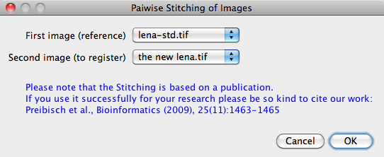 Shows the selection of input images.
The Pairwise Stitching first queries for two input images that you intend to stitch. They can contain rectangular ROIs which limit the search to those areas, however, the full images will be stitched together. Once you selected the input images it will show the actual dialog for the Pairwise Stitching. The dialog will depend on the dimensionality of the input images. Please note that RGB input images will be converted into 8-Bit composite images.
- Linear blending: In the overlapping area the intensity are smoothly adjusted between the two images.
- Average: In the overlapping area the average intensity between all images is computed (example source code).
- Median: In the overlapping area the median intensity of all images is computed.
- Max. Intensity: In the overlapping area the maximum intensity between all images is used int the output image.
- Min. Intensity: In the overlapping area the minimum intensity between all images is used int the output image.
- Overlay into Composite: all channels of all input images will be put into the output image as separate channels.
- Do not fuse images: no output images will be computed, just the overlap is computed.
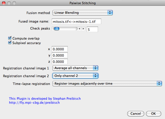 Shows the Pairwise Stitching dialog.
The number of peaks defines the number of maxima in the Phase Correlation Matrix which are examined. If the stitching was not correct increasing this number might help.
If you do not check compute overlap, the plugin will just apply the translation that can be inserted below.
If you check supixel accuracy, the plugin will compute a subpixel precise alignment between the two images (it hardly costs any computation time but some RAM). Furthermore, if subpixel localization is activated, linear interpolation will be used for the fusion. Otherwise no interpolation will be applied.
When choosing the registration channels you define which part of the data will be used to compute the overlap. It has no influence on how the data is fused.
If the input stacks are time-lapse images, you will have different choices on how to align over time:
- Apply registration of first time-point to all other time-points: The plugin will compute the stitching only for the first time-point and assume that this shift is correct for all time-points.
- Register images adjacently over time: The stitching will compute the shift between all images of all time-points, as well as of each image to the same image of the next time-point. A global optimization scheme will be used to minimize the global error and reject outliers. The parameters for this global optimization will be queried in an additional dialog.
- Register all images over all time-points globally (expensive!): The stitching will compute the shift between all time-points and all images which will take a considerable amount of time. A global optimization scheme will be used to minimize the global error and reject outliers. The parameters for this global optimization will be queried in an additional dialog.
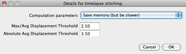 Shows the extra option for Pairwise Stitching when aligning all timepoints to each other.
If a global optimization is necessary for time-point registration another dialog will pop up to ask for more parameters:
- Computation parameters: If you choose Save memory (but be slower) the stitching will compute all pairwise correlations one after another. Although it is performed multi-threaded it is slower than computing as many pairwise correlations at the same time as processors are available done by the option Save computation time (but use more RAM).
- Max/avg displacement threshold: After the overlap between all individual tiles has been computed the global optimization computes an optimal arrangement of all tiles. After that, some image pairs will be placed different to each other compared to the individual alignment, which we call displacement. If there are no major alignment errors the average and maximal displacement will be below or around 1 pixel. If one of the individual alignment between two images was wrong, this pair will be displaced a lot in the global optimization as all other connecting tiles pull it towards the correct global position. If the maximal displacement is much higher than the average one it means that this individual alignment is most likely wrong and will be removed. Note: An image will just be removed if there is no link to another image any more.
- Absolute displacement threshold: Removes links between images if the absolute displacement is higher than this value.
Grid/Collection Stitching
This plugin is able to stitch an arbitrary collection or grid of images, it does not matter if it is 2d, 3d, 4d or 5d images as long as all images are of the same type. In contrast to the Pairwise Stitching of two images, this plugins will load (and potentially save) the images from/to harddisc.
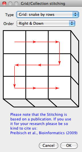 Shows the grid/collection selection dialog.
Please note that you should take the chance to give the Grid/Collection Stitching a clue of what the approximate layout of the tiles is if you can. This will reduce the computational effort significantly and is much more likely to succeed. If this is not possible, choose the option Unknown positions and the Stitching will try to figure out the correct alignment without any help.
The first dialog queries the type image collection or image grid that you want to assemble. For each major type there are typically several subtypes you can choose from. For an easier understanding each option is supported by a small figure:
- Grid: row-by-row: The images are arranged in a grid, one line after the other. After a line is finished the new one always starts at the same position as the previous line (carriage return, like reading a text).
- Right & Down: Start on the top left and go down line by line.
- Left & Down: Start on the top right and go down line by line.
- Right & Up: Start on the bottom left and go up line by line.
- Left & Up: Start on the bottom right and go up line by line.
- Grid: column-by-column: The images are arranged in a grid, one column after the other. After a column is finished the new one always starts at the same position as the previous column (carriage return).
- Down & Right: Start on the top left and go right column by column.
- Down & Left: Start on the top right and go left column by column.
- Up & Right: Start on the bottom left and go right column by column.
- Left & Up: Start on the bottom right and go left column by column.
- Grid: snake by rows: The images are arranged in a grid, one line after the other. After a line is finished the next line starts in reverse order at the position where the previous line ended (no carriage return, like a snake).
- Right & Down: Start on the top left and go right, then one line down, then left, then down, then right, …
- Left & Down: Start on the top right and go left, then one line down, then right, then down, then left, …
- Right & Up: Start on the bottom left and go right, then one line up, then left, then up, then right, …
- Left & Up: Start on the bottom right and go left, then one line up, then right, then up, then left, …
- Grid: snake by columns: The images are arranged in a grid, one column after the other. After a column is finished the next one starts in reverse order at the position where the previous one ended (no carriage return, like a snake).
- Down & Right: Start on the top left and go down, then one column right, then up, then right, then down, …
- Down & Left: Start on the top right and go down, then one column left, then up, then left, then down, …
- Up & Right: Start on the bottom left and go up, then one column right, then down, then right, then up, …
- Up & Left: Start on the bottom right and go up, then one column left, then down, then left, then up, …
- Filename defined positions: The approximate positions of each tile are encoded in the filename.
- Unknown positions: The positions of each tile are unknown and the Stitching will try to determine them.
- Positions from file: The approximate position of each tile is defined in an extra file or by the metadata.
- Defined by TileConfiguration: The next dialog will query for a tile configuration file that specifies the filenames as well as the approximate position of each tile in pixel coordinates. This is especially useful if the tiles are arranged in a way that is not covered by any of the other grid/snake options - or maybe also in z! You will find an example tile configuration file below. If you want to manually or automatically create such a file I suggest creating one using grid stitching (even if you do not have any image data) and changing it accordingly.
- Defined by meta data: Use this option if all tiles are stored in one big file that also contains the approximate stage positions in its meta data. When importing you will have the chance to further increase the overlap and define if the stage coordinates are calibrated or in pixel coordinates.
 Once you selected your type of acquisition a second dialog will pop up that is slightly different depending up on your first selection. Here, I will explain the dialog that is used for any grid as this is the most complex one.
The user has to define the grid size, that means how the input tiles are arranged (e.g. 7 x 7 image tiles). The tile overlap is a rough estimate. Note: Smaller overlap reduces computation time, but if the correct alignment is not found try increasing this value first.
The grid stitching assumes that the tiles which are arranged in any kind of grid are incrementally numbered. The First tile index i defines the number of the first tile in your approximate tile configuration (see figure above). Next, you have to choose the directory that contains the different tiles. Note: if you just have one big file containing all tiles, choose the option Positions from file -> Defined by meta data in the first dialog.
The next entry File name for tiles in the dialog is used to tell the plugin how to find the images which are in the grid (e.g. 49 different file names). Let’s assume the files are simply named like this:
tile_001.lsm tile_002.lsm …. tile_049.lsm
which translates to the following entry tile_{iii}.lsm. It tells the plugin where to put the increasing index number i, and furthermore to use leading zeros with a length of 3. If the tiles would be called tile_1.lsm tile_2.lsm …. tile_49.lsm, it would translate to tile_{i}.lsm.
If you select ‘Filename defined position / Defined by filename as type, the approximate coordinates in the grid should be part of the filename. Assuming your files are called:
tile_x01_y01.lsm tile_x02_y01.lsm …. tile_x10_y10.lsm
it would translate to the following pattern: tile_x{xx}_y{yy}.lsm.
The Output textfile name defines the text files that will contain the initial approximate grid layout and the final positions of each tile after registration.
The fusion methods are almost the same as the ones for the Pairwise Stitching, please check them out above.
The next three entries describe the behaviour of the global optimization:
- regression threshold: If the regression threshold between two images after the individual stitching are below that number they are assumed to be non-overlapping. Typical values for a good registration are over 0.7, however in noisy images with less content also small regression thresholds can be a correct overlap.
- max/avg displacement threshold: After the overlap between all individual tiles has been computed the global optimization computes an optimal arrangement of all tiles. After that, some image pairs will be placed different to each other compared to the individual alignment, which we call displacement. If there are no major alignment errors the average and maximal displacement will be below or around 1 pixel. If one of the individual alignment between two images was wrong, this pair will be displaced a lot in the global optimization as all other connecting tiles pull it towards the correct global position. If the maximal displacement is much higher than the average one it means that this individual alignment is most likely wrong and will be removed. Note: An image will just be removed if there is no link to another image any more.
- absolute displacement threshold: Removes links between images if the absolute displacement is higher than this value.
There are then a series of toggles you can now choose to enable or disable.
First, you can add tiles as ROIs, which will generate a ROI in the ImageJ RoiManager for each stitched tile. If possible, the ROI name will contain the source file for its corresponding tile, allowing easy identification of images of interest. This will also enable and select the ROI Picker tool, so you can select the ROI covering a desired visual area.
Next, you can choose whether to compute the overlap or trust the (approximate) location defined by the grid, the meta data or the tile configuration file.
The invert x and invert y options are extremely important if you know your dataset was collected with inverted coordinates in either of these axes. If your stitched image comes back with tiles appearing to be flipped horizontally and/or vertically, try enabling these options (as appropriate).
The ignore Z stage position can be useful if individual tiles for a given XY plane in your dataset were acquired at slightly different Z positions (e.g. on a sloping gradient). The stitching plugin relies on matching Z positions to define XY planes, so if your stitched image comes back with lots of empty space and tiles scattered between slices, try this option.
If you check supixel accuracy, the plugin will compute a subpixel precise alignment between the two images (it hardly costs any computation time but some RAM). Furthermore, if subpixel localization is activated, linear interpolation will be used for the fusion. Otherwise no interpolation will be applied.
 If downsample tiles is selected, a dialog will pop up during the stitching process allowing you to specify a new (smaller) image size. The current image size will be displayed at first. You can enter either a new scale (from 0-1) or a direct pixel value for the new height and width. A variety of interpolation algorithms can be selected. When you are happy with the downsampler settings, click ok and stitching will continue. Note that downsampling will occur before matching or fusion of tiles, so using this option can significantly speed up these operations and reduce the final fused image’s memory footprint.
Now, you can choose to open the input stacks as virtual stacks. This results in a significantly reduced memory consumption, however, it will consume more time to perform the computation.
Computation parameters: If you choose Save memory (but be slower) the stitching will compute all pairwise correlations one after another. Although it is performed multi-threaded it is slower than computing as many pairwise correlations at the same time as processors are available done by the option Save computation time (but use more RAM).
Finally, you can choose whether to display the result or write the fused image to disk. If you choose to write it to disk, it will require very little memory to do so as it writes it slice-by-slice. You can later on open this dataset virtually or partially and convert it back to a Hyperstack (Image › Hyperstacks › Stack to Hyperstack…). Writing it directly to disk, will, however, take more time than just displaying it.
Grid Collection/Stitching plugin
Please see the Grid/Collection Stitching Plugin page for a complete set of instruction on how to use Grid/Collection stitching in Fiji.
Problems, known issues and solutions
If the output is not correct
If the Grid/Collection Stitching is not able to create the correct output image you can do it yourself iteratively using the Pairwise Stitching plugin. You just start with the first two images and fuse them. Using ROIs on clearly similar areas you can force a correct alignment. Afterwards you fuse the result with the third image and so on. The biggest drawback apart from the time consumption is that you can only use Maximum Intensity as fusion method, otherwise the image will look weird. Furthermore it will consume more memory.
Problems loading the images
For loading microscopic images we use the LOCI Bioformats importer. If you experience problems loading files, convert them to TIFF before, it should be read fine.
Minimal number of z-sections
Three-dimensional stitching will not work for z-Stack size of smaller than 3 pixels. If you want to reconstruct such image from very thin tiles, duplicating of some of the stacks should solve the problem. Or you try to work just on the maximum/average intensity projections of the thin stacks.
Register different channels to each other
The plugin is not build to register different channels to each other. However, if you want to do that anyways simply convert channels into time-points and run it as if it was time-lapse registration. Afterwards you can convert it back. The easiest to achieve this is to use Image › Hyperstacks › Re-order hyperstack…
Timelapse alignment for Grid/Collection Stitching
You might notice that the Grid/Collection Stitching does not offer any options for time-lapse alignment although it does perform it. For now, it always uses the option Apply registration of first time-point to all other time-points (as available in Pairwise Stitching)
I have a known approximate arrangement for the tiles but it is not any of the grids
If you still have a known arrangement of tiles that is not covered by any of the grid methods, you can create yourself a tile configuration file which roughly describes the arrangement including the overlap. You can use this as input for the Grid/Collection stitching (option Positions from file -> Defined by TileConfiguration) to refine it and find the correct alignment. Here is an example TileConfiguration.txt:
# Define the number of dimensions we are working on
dim = 3
# Define the image coordinates (in pixels)
img_73.tif; ; (0.0, 0.0, 0.0)
img_74.tif; ; (409.0, 0.0, 0.0)
img_75.tif; ; (0.0, 409.0, 0.0)
img_76.tif; ; (409.0, 409.0, 0.0)
img_77.tif; ; (0.0, 818.0, 0.0)
img_78.tif; ; (409.0, 818.0, 0.0)
I want to define a different overlap for X and Y using a Grid-Layout
This option exists, but is disabled by default as it is likely only required in non-standard scenarios. You can enable it as follows using the script editor:
- File › New › Script
- Language › Beanshell
- type the following line:
plugin.Stitching_Grid.seperateOverlapY = true;
- click Run
From now on, there will be a second slider for the overlap in Y on the currently running Fiji instance.
I want to change the blending parameter for the fusion
You can change the fraction of the area that is blended using the scripting language. By default it is set to 0.2 (20%), but you can change it to anything between 0 and 1. You can do so using the script editor:
- File › New › Script
- Language › Beanshell
- type the following line to change it to e.g. 10%:
mpicbg.stitching.fusion.BlendingPixelFusion.fractionBlended = 0.1;
- click Run
From now on, the blending will work only on the outer 10% of each tile. This change is only valid for the currently running Fiji instance.
I want to ignore the movement of tiles in Z
Sometimes people only want to stitch in x and y, but not in z. There is an ad-hoc way of achieving this which will only ignore the translation in z at the time of the global optimization and fusion. If this turns out to be more useful, I will integrate more properly.
You can activate the option using the script editor:
- File › New › Script
- Language › Beanshell
- type the following line:
mpicbg.stitching.GlobalOptimization.ignoreZ = true;
- click Run
From now on, any shift in z will be ignored for 3d acquisitions. This change is only valid for the currently running Fiji instance.
Results & Computation time

The figure shows stitched images of 3D confocal tiles. (A) shows a Drosophila melanogaster pupae expressing a GFP reporter under the regulation of the yellow gene, imaged few hours before eclosion using a 4× dry lens on an Optiphot confocal microscope (Nikon). It was stitched from three image stacks arranged in a 1 × 3 grid (Table 1 first row). The maximum intensity projection is shown. (B) shows the Drosophila larval nervous system stained with three dyes, stitched from a grid of 2 × 3 RGB images (see table 1 second row), the maximum intensity projection is shown. (C) shows a zone in the dorsal telencephalon of human embryonic tissue from week 17 post conception, incubated for 24 hours at 37°C in DiI. It was imaged using a 63×/1.4 objective on Zeiss LSM 510 equipped with a motorized stage. The final image was created from 24 image stacks arranged in a 4 × 6 grid (see table 1 third row), slice 18 is shown. Special thanks to Nicolas Gompel, James W. Truman, Simone Fietz and Wieland B. Huttner for providing the images.
For interactive examples of these datasets have a look here.
| tiles | individual tile dimension | output image dimension | output image size | computation time | min/avg/max displacement |
|---|---|---|---|---|---|
| 3 | 1024×1024×42 | 1097×2345×43 | 108 MB (8 Bit) | 0:42 min | 0.00/0.00/0.00 px |
| 6 | 512×512×86 | 975×1425×86 | 350 MB (RGB) | 1:20 min | 0.60/0.77/1.05 px |
| 24 | 1024×1024×68 | 3570×5211×70 | 1200 MB (8 Bit) | 22:43 min | 0.49/0.76/0.99 px |
| 72 | 512×512×122 | 3391×3847×145 | 1850 MB (8 Bit) | 43:10 min | 0.00/0.39/0.64 px |
| 63 | 1024×1024×92 | 6088×7667×119 | 5424 MB (8 Bit) | 178:57 min | 0.00/0.66/1.18 px |
The Table shows examples of stitched data computed on an Intel® Quad-Core CPU machine with 2.67GHz and 24GB of RAM. The global alignments of all stitchings have an average error below 1 px, the displacements in row 1 are zero because the two alignments are independent of each other. Note that the computation time scales roughly linearly with the output image size.
Contact
For any type of comment, questions or input please write to preibischs@janelia.hhmi.org or visit my homepage.
Acknowledgements
The Stitching depends on quite a few libraries. I want to thank all the authors for their support and help:
- Mines Java Toolkit (JTK): Efficient 1-dimensional FFT implementation by Dave Hale.
- MPI-CBG Transformation Package by Stephan Saalfeld.
- Imglib: N-dimensional image processing library for Java by Stephan Preibisch and Stephan Saalfeld (now superseded by ImgLib2).
- fiji-lib and Fiji_Plugins: Fiji libraries by Johannes Schindelin.
- Bio-Formats Java library for reading and writing life sciences image file formats. I want to especially thank Curtis Rueden and Melissa Linkert.
Additionally, I want to thank the following people for discussions, providing images and pushing me to develop and continuously improve the Stitching plugins:
Danielle Bower, Albert Cardona, Nicolas Gompel, Wieland Huttner, Gregory Jefferis, Arnim Jenett, Tom Kazimiers, David Koos, Jan Peychl, Pavel Tomancak, James Truman, Nicholas Weiler and Daniel James White.
See Also
- The Publication on the Stitching Plugin, S. Preibisch, S. Saalfeld, P. Tomancak (2009) Globally optimal stitching of tiled 3D microscopic image acquisitions”, Bioinformatics, 25(11):1463-1465. PDF
- TrakEM2 for non-destructive stitching with floating, adjustable images.
- XuvTools similar stitching software (but you cannot access XuvTools’ source code freely) from the University of Freiburg and the abstract of the accompying publication