The content of this page has not been vetted since shifting away from MediaWiki. If you’d like to help, check out the how to help guide!
This software is a tool for the tracking of low-light sub-resolution objects in fluorescent microscopy. It can be applied in other fields as well. The plugin implements the localization algorithm described in the following paper:
Installation of the plugin
The plugin can be quickly installed via the projects update site. This is unfortunately may not possible if you are using a Fiji version installed via package management system. If you encounter this problem, please use the Fiji version obtainable here.
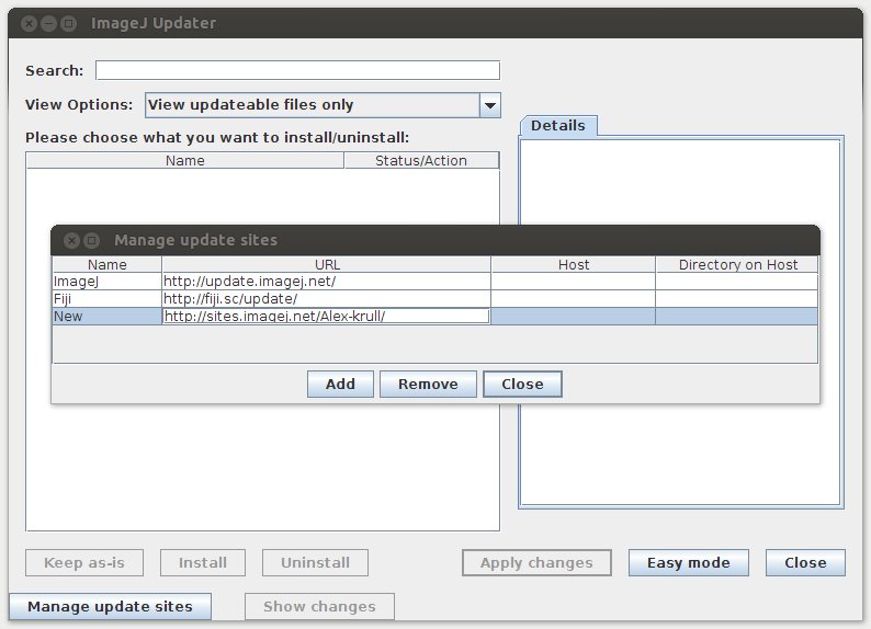
Add the project’s update site to your Fiji installation
Please refer to the tutorial on how to add our update site to your Fiji installation. Our update site has the following URL:
` **http://sites.imagej.net/Alex-krull/`**
Install the required files
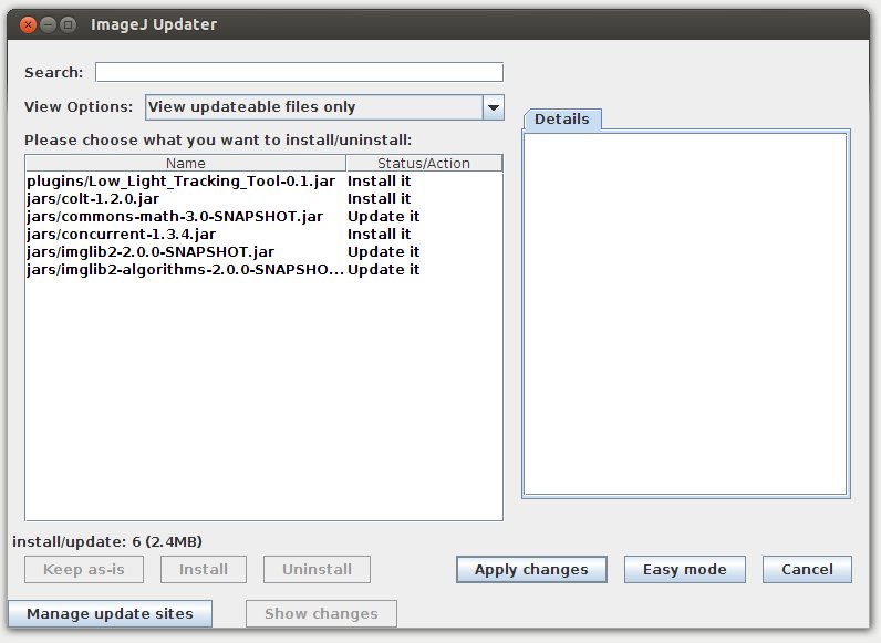
Install or update all 6 items shown above by hitting Apply changes. Please restart Fiji afterwards.
Startup
Load the data
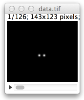
To begin use Fiji to load the data to be used for tracking. Use whichever method you prefer in Fiji. The LLTT-plugin will work with 8-bit, 16-bit and 32-bit-float stacks. Moreover you can use 3D and multichannel hyperstacks. If you want to try the LLTT-plugin but do not have the right data at hand, you can download a file with sample data here: 
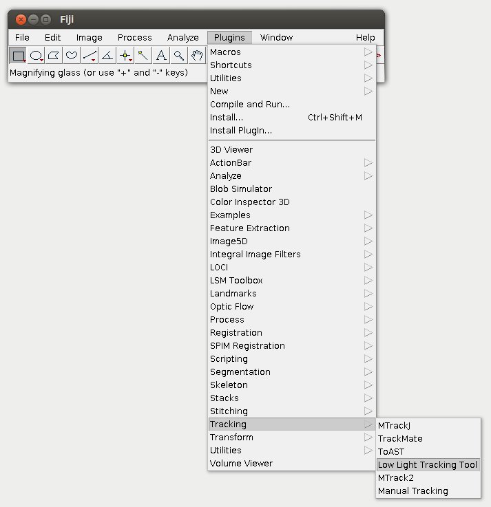
Start the LLTT-plugin
After the data is loaded, start the plugin by clicking:
Plugins › Tracking › Low Light Tracking Tool
Set global options
Upon startup of the plugin you will be asked to enter three values.
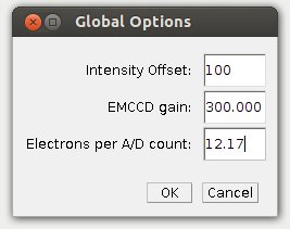
They are:
Intensity Offset
Cameras used in microscopy often add a bias or Intensity Offset in order to avoid potentially negative values caused by read out noise. This quantity should be specified here, in order to obtain optimal tracking results.
EMCCD gain
If you are using an EMCCD camera you should specify the mean EMCCD gain that was used. Otherwise set it to 1.0.
Electrons per A/D count
Finally you have to provide the ratio at which the analog digital unit in your camera converts photo electrons into A/D counts.
Please consult you camera’s specs sheet to obtain this information. The EMCCD gain and Electrons per A/D count are required for tracking with the EMCCD-GaussianML method. The GaussianML method uses these values to correct the measured flux of the object and background.
The User Interface
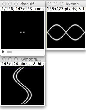
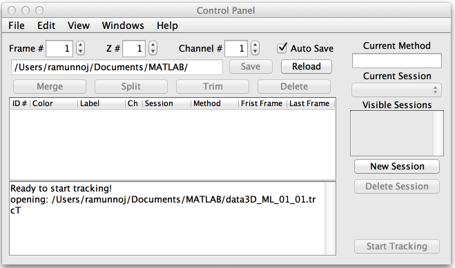
The different windows
When the plugin starts on a 2D image stack you have three windows and the control panel. The main data window lets you move through the slices like normal. On the sides you see the two kymographs, which makes it easier to see movement over time. The control window will help you to organize your tracking activity.
If you would like the windows to become larger or smaller, change the size of the main data window and then select Arrange Windows, from the View menu. Alternatively you can use the hot-key ⌃ Ctrl + W (when the focus is on the control panel) or W (when the focus is on one of the other windows). This will also organize the windows if they have become scattered.
If you close some of the windows you can bring them back using the Windows menu in the control panel. If you close the control panel, this will terminate the program. Don’t forget to Save your results before.
Navigation
The yellow lines in the kymographs indicate what frame you are currently working on. If you work with 3D data yellow lines in the side projections indicate what slice you are looking at. There are three ways of navigating through your stack or hyper stack:
- You can use ImageJ/Fiji slider controls below the main window.
- You can set frame number, slice number and channel number in the control window.
- You can use your middle mouse button to click directly into one of the kymographs to set the frame number. If you are working with 3D data you can click into one of the side projections with your middle mouse button to set the slice number.
Basic tracking
Create session
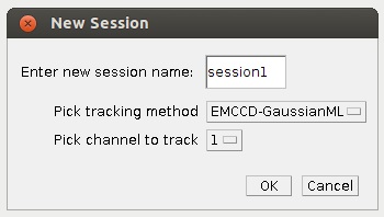
Click on the New Session button or select from the menu. The New session window opens. Here you can pick a name for the session as well as the channel you want to track on. Finally you can choose your tracking method.
Choose a tracking method
There are currently two tracking algorithms available:
GaussianML
This algorithm implements the maximum likelihood estimator based on a shot noise model. This means it considers the statistics of photon distribution in the image generation process to find the optimal location estimate. In our publication this is referred to as the inner loop.
EMCCD-GaussianML
This algorithm implements the maximum likelihood estimator based on a more sophisticated model which in addition includes the stochastic amplification process in an EMCCD camera. We have shown, that it yields more accurate results in situations with low light levels. In our publication this algorithm is referred to as the Nested Maximum Likelihood Algorithm.
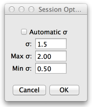
Pick session options
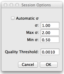
After clicking OK, a new window will open. In this window you can choose a σ value, which denotes the standard deviation (in pixels) of the Gaussian used to approximate the Point Spread Function (PSF) of the tracked objects. If you select Automatic σ, this value is used only as initialization. In this case Min and Max are used as bounds for the estimation. These values will be the default values for all new traces you make in this session.
You also can set your quality threshold. Smaller numbers are higher quality, while larger numbers are lower quality but faster.
Fixed σ can be more stable and also faster, this is more so for 3D data. All settings can later be altered by clicking on Session Options, under Edit.
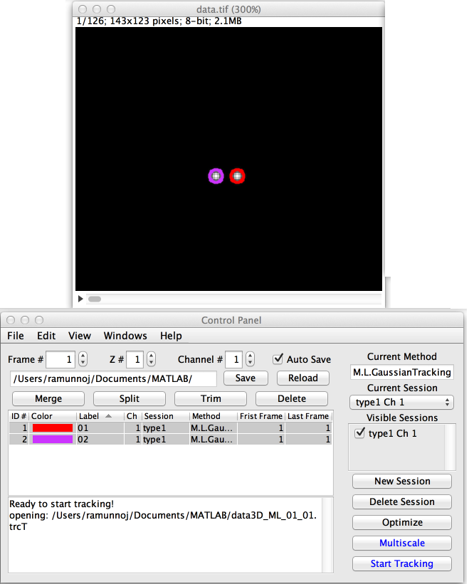
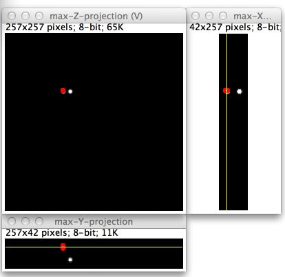
Adding objects to track
To add an object in order to track it, make sure the cross hair icon in the Fiji toolbar is selected and then double click roughly on the object you would like to track in the main window. This new object is represented as a circle. An accordant entry will appear in the table in the control panel representing the objects trace. You can select objects by clicking on them in the control panel or directly in the main window. You can then move them around, using drag and drop or edit them. Multiple objects can be selected by holding ⇧ Shift when selecting.
You can change a trace’s label by clicking on the text in the label field or change the color by clicking on the colored area.
Edit individual objects
The default settings made in the session options dialog will only effect new traces. If at this point you find that the parameters you picked were less ideal you can change the parameters with the Edit Object selection from the Edit menu.
The settings you make here will effect the selected object in the very frame you are looking at.
Start tracking
Only the highlighted objects will be tracked. So in the example above both are highlighted and will be tracked at the same time. To start tracking select at least one trace and click on the Start tracking button or hit the hot-key G. The software will start at the frame you are currently looking at and continue with the following frames until the end of the movie or until you hit G again or click on Stop tracking
Objects that are very close to each other should generally be tracked jointly by selecting them both before starting to track. Objects which are far away from each other should be tracked in individually one after the other.
Working with tracking results
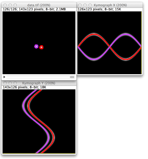
You can watch the trace fill in the kymograph line as the tracking is in progress. If you see the tracking looks incorrect and lost the object, you can click on Stop Tracking and adjust the object location and the software will resume from the new starting point.
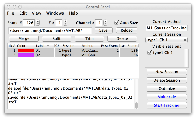
The table now contains more information, with the first frame of the trace, and the last frame. Double clicking on the ID# of the object will jump the frame number to the beginning and end of the trace.
Saving and loading
The tracking results are already saved automatically by default. You can turn that off by un-checking the Auto Save box. The results can than be saved using the Save button. They are by default stored in the directory of the image stack you are working on. The file format is described below. When you start the plugin again with the same data file your results will be automatically loaded. You can also reload previously tracked data and undo any unsaved changes by pressing the reload button. If you want to open data which is stored in a different location you can load it by clicking on the address bar and navigating to the data’s location. You can then re-track, or examine the data.
Deleting and manipulating traces and sessions
Using the Merge, Split, Trim and Delete buttons allows you to edit your traces by combining or deleting them. Sessions can be deleted using the ‘Delete Session’ button.
Merging
One useful application for merging of two traces is if your object disappears periodically but you know that it is not a new object, and would like to combine the two separate traces you create. You have to select at least two traces to merge them.
Splitting
Splitting will do the opposite of merging and make two traces out of one by cutting it at the current frame.
Trimming
Trimming has the same effect as splitting but it keeps only the first part, while discarding the second.
Deletion
When you delete a trace or a session you will be asked whether to delete the corresponding files as well. If you delete the files the traces will be permanently (!) removed. If you don’t delete them, they can be restored using the reload button.
Changes done by Merge, Split and Trim can also be undone in this way. They are made permanent only when you hit the Save button or start tracking with the Autosave option activated.
Advanced features
3D data
The plugin can be used to track objects in 3D volumes as well. When working with 3D data you will be asked upon startup to provide the ΔZ ratio in addition to the Intensity Offset, EMCCD gain and Electrons per A/D count.
The ΔZ ratio is the slice thickness divided by the pixel width. This value is only used for 3D data. Example: My pixel size for my data is 100 nm and my slice thickness is 200 nm. I would then enter a value of 2.
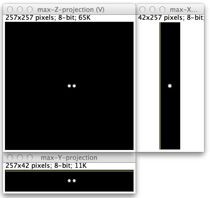
3D data is very similar to 2D data, there are just a few more windows that open when you start. The data window and the kymographs appears, but a second set of windows appear. A max Z projection window and max Y and X projects. The side projections are useful to place your starting tracking in the correct slice. So before clicking on the object in the data window, change the z to the correct plane first.
Otherwise, tracking function is the same. It is best to optimize the σ-value for 3D tracking and then use a fixed value to increase speed.
Using multiscale tracking for fast moving objects
If you are trying to track fast moving objects that move over a big distance between two frames, the software might loose the target at some point. To avoid this you can use multiscale tracking, which uses iterative smoothing and down-sampling to find the target in each frame. To start tracking in multiscale mode hit the Multiscale.
You can change the default behavior in the edit menu.
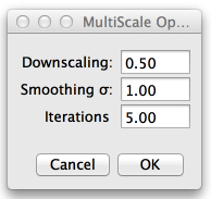
The algorithm builds a pyramid by repetitively smothing the image with a Gaussian kernel with the standard deviation given in the Smoothing σ field and than down-sampling it by a factor set in the Downscaling field. The pyramid’s hight (i.e. the number of repetitions) can be set in the iterations field. Localization is than first performed on the top level of the pyramid and repeated until its bottom, which is the original image.
Tips
- If you want to be able to see the original image data and find your tracking results get in the way, you use the hot-key P or ⌃ Ctrl + P respectively to hide all overlays (all circles lines and cross-hairs drawn on top of the image).
- If some of the windows appear to bright or to dark use View › Adjust Brightness/Contrast to correct them.
- You can use File › Export images to export a sequence of image with the tracking results drawn on top of them. You can use this to create a movie in order to demonstrate your tracking results. In your working directory a new folder named movieMain will be created and filled with images.
- If you have multichannel data, each channel needs its own session. You can select which sessions are visible by checking their boxes in the Visible Sessions list. You can use the current session drop down menu to switch between sessions.
- You can zoom into the kymographs by moving the cursor over the kymograph window and holding down ⇧ Shift, while using the scroll wheel on the mouse.
- You can use the optimize button. This will perform the tracking of the selected objects on the single frame you are looking at. You can use this for example with Automatic σ turned on to determine the size of the target’s PSF on a single frame.
Hot-keys
There are several hot-keys you can use. You can find the key to press in the menus of the control panel. When the focus is on the control panel you have to press ⌃ Ctrl to access hotkeys. When the focus is on one of the other windows this is not necessary.
File format
The tracking results are stored in text files with the ending ‘.trcT’. Each file holds the result of one trace. The structure of the file name is the following:
<name of image file>_<name of session>_<label of trace>_<id of trace>.trcT
The files are created in the working directory. Each file begins with some lines starting with #. These lines store information for the tracking program they will be ignored by most programs like MATLAB or gnuplot potentially used to further analyze the data. This meta information is followed by columns of data holding the actual tracking results. The columns have the following meaning:
- column 1 frame number
- column 2 trace id
- column 3 x-position in pixels
- column 4 y-position in pixels
- column 5 z-position in pixels
- column 6 σ, the standard deviation (in x and y) of the Gaussian used as Point Spread Function PSF
- column 7 the standard deviation (in z) of the Gaussian used as Point Spread Function PSF
- column 8 the maximum value of σ in case σ is determined automatically
- column 9 boolean value indicating if σ was fixed (1) or determined automatically (0)
- column 10 boolean value indicating if object was assumed to be coupled (assumed to have the same flux and σ) with others.
- column 11 the estimated flux in photons
- column 12 the estimated background flux in photons per pixel
- column 13 the total estimated background flux in the considered window in photons
- column 14 the number of pixels in the considered window
- column 15 the fraction of flux in the considered window assumed to belong to the tracked object
- column 16 the total estimated flux in the considered window
Example Data
This link contains the data used to generate this tutorial, and a two channel 3D data set to try. Example_Data.zip
License
This program is free software; you can redistribute it and/or modify it under the terms of the GNU General Public License as published by the Free Software Foundation (http://www.gnu.org/licenses/gpl.txt).
This program is distributed in the hope that it will be useful, but WITHOUT ANY WARRANTY; without even the implied warranty of MERCHANTABILITY or FITNESS FOR A PARTICULAR PURPOSE. See the GNU General Public License for more details.
Colt library
We redistribute packages from the colt library. They have the following licenses:
Packages cern.colt* , cern.jet*, cern.clhep Copyright (c) 1999 CERN - European Organization for Nuclear Research.
Permission to use, copy, modify, distribute and sell this software and its documentation for any purpose is hereby granted without fee, provided that the above copyright notice appear in all copies and that both that copyright notice and this permission notice appear in supporting documentation. CERN makes no representations about the suitability of this software for any purpose. It is provided “as is” without expressed or implied warranty.
Packages hep.aida.*
Written by Pavel Binko, Dino Ferrero Merlino, Wolfgang Hoschek, Tony Johnson, Andreas Pfeiffer, and others. Check the FreeHEP homepage for more info. Permission to use and/or redistribute this work is granted under the terms of the LGPL License, with the exception that any usage related to military applications is expressly forbidden. The software and documentation made available under the terms of this license are provided with no warranty.