This page shows eight increasingly complex examples of how to program with ImgLib2. The intention of these examples are not to explain ImgLib2 concepts, but rather to give some practical hints how to work with the library and to grasp the principles in a learning-by-doing way.
Jupyter notebook
This tutorial is also available in Jupyter notebook form here!
Introduction & required files
All examples presented on this page are always entire classes including a main method to run them. Simply copying them into your favorite editor (e.g. the Script Editor) and compile & run them. The required Java libraries (jar files) are part of ImageJ2 and can be found in ImageJ2.app/jars/:
- imglib2 (the core)
- imglib2-algorithm (algorithms implemented in ImgLib2)
- imglib2-algorithm-gpl (for example 6b and 6c: GPL-licensed algorithms implemented in ImgLib2—ships with Fiji only, not plain ImageJ2, for licensing reasons)
- imglib2-ij (the ImageJ interaction)
- imglib2-realtransform (for example 8)
- scifio (for reading and writing files)
- ij (ImageJ core, used for display)
Alternately, you can access the examples from the ImgLib-tutorials Git repository. After cloning the source code, open the project in your favorite IDE. See Developing ImgLib2 for further details.
Example 1 - Opening, creating and displaying images
The first example illustrates the most basic operations of opening, creating, and displaying image content in ImgLib2. It will first focus on entires images (Img<T>), but also show how to display subsets only.
Example 1a - Wrapping ImageJ images
If you are already an ImageJ programmer, you might find it the easiest way to simply wrap an ImageJ image into ImgLib2. Here, the data is not copied, so editing the image in ImgLib2 will also modify the ImageJ ImagePlus.
Internally, we use a compatibility Img to represent the data which is as fast as ImageJ but in the case of higher dimensionality (>2d) is slower than ImgLib2 can do with the ArrayImg. Furthermore you are limited in dimensionality (2d-5d), in the type of data (UnsignedByteType, UnsignedShortType, FloatType and ARGBType) and maximal size of each 2d-plane (max. 46000x46000).
import ij.ImageJ; import ij.ImagePlus; import ij.io.Opener; import java.io.File; import net.imglib2.img.ImagePlusAdapter; import net.imglib2.img.Img; import net.imglib2.img.display.imagej.ImageJFunctions; import net.imglib2.type.NativeType; import net.imglib2.type.numeric.NumericType; /** * Opens a file with ImageJ and wraps it into an ImgLib {@link Img}. * * @author Stephan Preibisch * @author Stephan Saalfeld */ public class Example1a { // within this method we define <T> to be a NumericType (depends on the type of ImagePlus) // you might want to define it as RealType if you know it cannot be an ImageJ RGB Color image public < T extends NumericType< T > & NativeType< T > > Example1a() { // define the file to open File file = new File( "DrosophilaWing.tif" ); // open a file with ImageJ final ImagePlus imp = new Opener().openImage( file.getAbsolutePath() ); // display it via ImageJ imp.show(); // wrap it into an ImgLib image (no copying) final Img< T > image = ImagePlusAdapter.wrap( imp ); // display it via ImgLib using ImageJ ImageJFunctions.show( image ); } public static void main( String[] args ) { // open an ImageJ window new ImageJ(); // run the example new Example1a(); } }
Example 1b - Opening an ImgLib2 image
The typical way to open an image in ImgLib2 is to make use of the SCIFIO importer. Below you see two examples of how to open an image as (a) its own type (e.g. UnsignedByteType) and (b) as float (FloatType). For (a) we assume, however, that the file contains some real valued numbers as defined by the interface RealType. Color images are opened as well and color is represented as its own dimension (like in the ImageJ Hyperstacks).
Note that for (a) we use an ArrayImg to hold the data. This means the data is held in one single java basic type array which results in optimal performance. The absolute size of image is, however, limited to 2^31-1 (~2 billion) pixels. The type of Img to use is set by passing an ImgOptions configuration when calling the ImgOpener.
In (b) we use a CellImg instead. It partitions the image data into n-dimensional cells each holding only a part of the data. Further, SCIFIO takes care of caching cells in and out of memory as needed, greatly reducing the memory requirement to work with very large images.
The SCIFIO importer also requires Types that implement NativeType, which means it is able to map the data into a Java basic type array. All available Types until now are implementing NativeType, if you want to work with some self-developed Type it would be easiest to copy the opened Img afterwards. Please also note that until now, the only Img that supports non-native types is the ListImg which stores every pixel as an individual object!
Important: it does not matter which type of Img you use to hold the data as we will use Iterators and RandomAccesses to access the image content. It might be, however, important if you work on two Img at the same time using Iterators, see Example2.
import ij.ImageJ; import io.scif.config.SCIFIOConfig; import io.scif.config.SCIFIOConfig.ImgMode; import io.scif.img.ImgIOException; import io.scif.img.ImgOpener; import java.io.File; import net.imglib2.img.Img; import net.imglib2.img.display.imagej.ImageJFunctions; import net.imglib2.type.NativeType; import net.imglib2.type.numeric.RealType; /** * Opens a file with SCIFIO's ImgOpener as an ImgLib2 Img. */ public class Example1b { // within this method we define <T> to be a RealType and a NativeType which means the // Type is able to map the data into an java basic type array public < T extends RealType< T > & NativeType< T > > Example1b() throws ImgIOException { // define the file to open File file = new File( "DrosophilaWing.tif" ); String path = file.getAbsolutePath(); // create the ImgOpener ImgOpener imgOpener = new ImgOpener(); // open with ImgOpener. The type (e.g. ArrayImg, PlanarImg, CellImg) is // automatically determined. For a small image that fits in memory, this // should open as an ArrayImg. Img< T > image = ( Img< T > ) imgOpener.openImgs( path ).get( 0 ); // display it via ImgLib using ImageJ ImageJFunctions.show( image ); // create the SCIFIOConfig. This gives us configuration control over how // the ImgOpener will open its datasets. SCIFIOConfig config = new SCIFIOConfig(); // If we know what type of Img we want, we can encourage their use through // an SCIFIOConfig instance. CellImgs dynamically load image regions and are // useful when an image won't fit in memory config.imgOpenerSetImgModes( ImgMode.CELL ); // open with ImgOpener as a CellImg Img< T > imageCell = ( Img< T > ) imgOpener.openImgs( path, config ).get( 0 ); // display it via ImgLib using ImageJ. The Img type only affects how the // underlying data is accessed, so these images should look identical. ImageJFunctions.show( imageCell ); } public static void main( String[] args ) throws ImgIOException { // open an ImageJ window new ImageJ(); // run the example new Example1b(); } }
Example 1c - Creating a new ImgLib2 image
Another important way to instantiate a new ImgLib2 Img is to create a new one from scratch. This requires you to define its Type as well as the ImgFactory to use. It does additionally need one instance of the Type that it is supposed to hold.
Once you have one instance of an Img, it is very easy to create another one using the same Type and ImgFactory, even if it has a different size. Note that the call img.firstElement() returns the first pixel of any Iterable, e.g. an Img.
import ij.ImageJ; import net.imglib2.img.Img; import net.imglib2.img.ImgFactory; import net.imglib2.img.cell.CellImgFactory; import net.imglib2.img.display.imagej.ImageJFunctions; import net.imglib2.type.numeric.real.FloatType; /** * Create a new ImgLib2 Img of Type FloatType */ public class Example1c { public Example1c() { // create the ImgFactory based on cells (cellsize = 5x5x5...x5) that will // instantiate the Img final ImgFactory< FloatType > imgFactory = new CellImgFactory<>( new FloatType(), 5 ); // create an 3d-Img with dimensions 20x30x40 (here cellsize is 5x5x5)Ø final Img< FloatType > img1 = imgFactory.create( 20, 30, 40 ); // create another image with the same size // note that the input provides the size for the new image as it implements // the Interval interface final Img< FloatType > img2 = imgFactory.create( img1 ); // display both (but they are empty) ImageJFunctions.show( img1 ); ImageJFunctions.show( img2 ); } public static void main( String[] args ) { // open an ImageJ window new ImageJ(); // run the example new Example1c(); } }
Example 1d - Displaying images partly using Views
By using the concept of Views it is possible to display only parts of the image, display a rotated view, and many more cool things. Note that you can also concatenate them. Views are much more powerful than shown in this example, they will be increasingly used throughout the examples.
A View almost behaves similar to an Img, and in fact they share important concepts. Both are RandomAccessible, and Views that are not infinite are also an Interval (i.e. those Views have a defined size) and can therefore be made Iterable (see example 2c). In ImgLib2, all algorithms are implemented for abstract concepts like RandomAccessible, Iterable or Interval. This enables us, as can be seen below, to display a View the exact same way we would also display an Img.
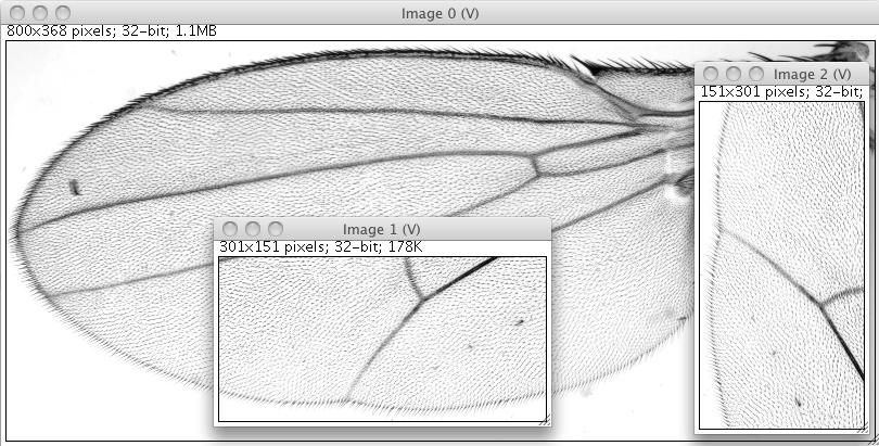 Shows the original image, the View of an interval, as well as the by 90 degree rotated version of the view. Note that only the original image in kept in memory, both Views are completely virtual.
import ij.ImageJ; import io.scif.img.IO; import io.scif.img.ImgIOException; import net.imglib2.RandomAccessibleInterval; import net.imglib2.img.Img; import net.imglib2.img.display.imagej.ImageJFunctions; import net.imglib2.type.numeric.real.FloatType; import net.imglib2.view.Views; /** * Open an {@code ArrayImg<FloatType>} and display partly and rotated */ public class Example1d { public Example1d() throws ImgIOException { // open file as float with SCIFIO Img< FloatType > img = IO.openImgs( "DrosophilaWing.tif", new FloatType() ).get( 0 ); // display image ImageJFunctions.show( img ); // use a View to define an interval (min and max coordinate, inclusive) to display RandomAccessibleInterval< FloatType > view = Views.interval( img, new long[] { 200, 200 }, new long[]{ 500, 350 } ); // display only the part of the Img ImageJFunctions.show( view ); // or the same area rotated by 90 degrees (x-axis (0) and y-axis (1) switched) ImageJFunctions.show( Views.rotate( view, 0, 1 ) ); } public static void main( String[] args ) throws ImgIOException { // open an ImageJ window new ImageJ(); // run the example new Example1d(); } }
Example 2 - How to use Cursor, RandomAccess and Type
The following examples illustrate how to access pixels using Cursor and RandomAccess, their basic properties, and how to modify pixel values using Type.
Accessing pixels using a Cursor means to iterate all pixels in a way similar to iterating Java collections. However, a Cursor only ensures to visit each pixel exactly once, the order of iteration is not fixed in order to optimize the speed of iteration. This implies that that the order of iteration on two different Img is not necessarily the same, see example 2b! Cursors can be created by any object that implements IterableInterval, such as an Img. Views that are not infinite can be made iterable (see example 2c). Note that in general a Cursor has significantly higher performance than a RandomAccess and should therefore be given preference if possible.
In contrast to iterating image data, a RandomAccess can be placed at arbitrary locations. It is possible to set them to a specific n-dimensional coordinate or move them relative to their current position. Note that relative movements are usually more performant. A RandomAccess can be created by any object that implements RandomAccessible, like an Img or a View.
Localizable is implemented by Cursor as well as RandomAccess, which means they are able to report their current location. However, for Cursor we differentiate between a LocalizingCursor and a normal Cursor. A LocalizingCursor updates his position on every move, no matter if it is queried or not whereas a normal Cursor computes its location on demand. Using a LocalizingCursor is more efficient if the location is queried for every pixel, a Cursor will be faster when localizing only occasionally.
The Sampler interface implemented by Cursor and RandomAccess provides access to the Type instance of the current pixel. Using the Type instance it is possible to read and write its current value. Depending on the capabilities of the Type more operations are available, e.g. +,-,*,/ if it is a NumericType.
Note that IterableInterval implements the java.lang.Iterable interface, which means it is compatible to specialized Java language constructs:
// add 5 to every pixel
for ( UnsignedByteType type : img )
type.add( 5 );
Example 2a - Duplicating an Img using a generic method
The goal of this example is to make a copy of an existing Img. For this task it is sufficient to employ Cursors. The order of iteration for both Img’s will be the same as they are instantiated using the same ImgFactory. It is possible to test if two IterableInterval have the same iteration order:
boolean sameIterationOrder =
interval1.iterationOrder().equals( interval2.iterationOrder() );
The copy method itself is a generic method, it will work on any kind of Type. In this particular case it works on a FloatType, but would also work on anything else like for example a ComplexDoubleType. The declaration of the generic type is done in the method declaration:
public < T extends Type< T > > Img< T > copyImage( ... )
< T extends Type< T > > basically means that T can be anything that extends Type. These can be final implementations such as FloatType or also intermediate interfaces such as RealType. This, however, also means that in the method body only operations supported by Type will be available. Note that the method returns a T, which also means that in the constructor from which we call method it will also return an Img<FloatType> as we provide it with one.
import ij.ImageJ; import io.scif.img.IO; import io.scif.img.ImgIOException; import net.imglib2.Cursor; import net.imglib2.img.Img; import net.imglib2.img.display.imagej.ImageJFunctions; import net.imglib2.type.Type; import net.imglib2.type.numeric.real.FloatType; /** * Here we want to copy an Image into another one using a generic method * * @author Stephan Preibisch * @author Stephan Saalfeld */ public class Example2a { public Example2a() throws ImgIOException { // open with SCIFIO as a FloatType Img< FloatType > img = IO.openImgs( "DrosophilaWing.tif", new FloatType() ).get( 0 ); // copy the image, as it is a generic method it also works with FloatType Img< FloatType > duplicate = copyImage( img ); // display the copy ImageJFunctions.show( duplicate ); } /** * Generic, type-agnostic method to create an identical copy of an Img * * @param input - the Img to copy * @return - the copy of the Img */ public < T extends Type< T > > Img< T > copyImage( final Img< T > input ) { // create a new Image with the same properties // note that the input provides the size for the new image as it implements // the Interval interface Img< T > output = input.factory().create( input ); // create a cursor for both images Cursor< T > cursorInput = input.cursor(); Cursor< T > cursorOutput = output.cursor(); // iterate over the input while ( cursorInput.hasNext()) { // move both cursors forward by one pixel cursorInput.fwd(); cursorOutput.fwd(); // set the value of this pixel of the output image to the same as the input, // every Type supports T.set( T type ) cursorOutput.get().set( cursorInput.get() ); } // return the copy return output; } public static void main( String[] args ) throws ImgIOException { // open an ImageJ window new ImageJ(); // run the example new Example2a(); } }
Example 2b - Duplicating an Img using a different ImgFactory
WARNING: The copyImageWrong method in this example makes a mistake on purpose! It intends to show that the iteration order of Cursors is important to consider. The goal is to copy the content of an ArrayImg (i.e. an Img that was created using an ArrayImgFactory) into a CellImg. Using only Cursors for both images will have a wrong result as an ArrayImg and a CellImg have different iteration orders. An ArrayImg is iterated linearly, while a CellImg is iterate cell-by-cell, but linearly within each cell.
 Shows the result if two Cursors are used that have a different iteration order. Here we are wrongly copying an ArrayImg (left) into a CellImg (right).
The correct code for the copy-method (in copyImageCorrect) requires the use of a RandomAccess. We use a Cursor to iterate over all pixels of the input and a RandomAccess which we set to the same location the output. Note that the setPosition() call of the RandomAccess directly takes the Cursor as input, which is possible because Cursor implements Localizable. Please also note that we use a LocalizingCursor instead of a normal Cursor because we need the location of the Cursor at every pixel.
import ij.ImageJ; import io.scif.img.IO; import io.scif.img.ImgIOException; import net.imglib2.Cursor; import net.imglib2.RandomAccess; import net.imglib2.img.Img; import net.imglib2.img.ImgFactory; import net.imglib2.img.array.ArrayImgFactory; import net.imglib2.img.cell.CellImgFactory; import net.imglib2.img.display.imagej.ImageJFunctions; import net.imglib2.type.Type; import net.imglib2.type.numeric.real.FloatType; /** * Here we want to copy an ArrayImg into a CellImg using a generic method, * but we cannot do it with simple Cursors as they have a different iteration order. * * @author Stephan Preibisch * @author Stephan Saalfeld */ public class Example2b { public Example2b() throws ImgIOException { // open with ImgOpener. In addition to using ImgOptions, we can directly // pass an ImgFactory to the ImgOpener. This bypasses the Img selection // heuristic and allows custom ImgFactory implementations to be used Img< FloatType > img = IO.openImgs( "DrosophilaWing.tif", new ArrayImgFactory<>( new FloatType() ) ).get( 0 ); // copy the image into a CellImg with a cellsize of 20x20 // Img< FloatType > duplicate = copyImageWrong( img, new CellImgFactory<>( new FloatType(), 20 ) ); Img< FloatType > duplicate = copyImageCorrect( img, new CellImgFactory<>( new FloatType(), 20 ) ); // display the copy and the original ImageJFunctions.show( img ); ImageJFunctions.show( duplicate ); } /** * WARNING: This method makes a mistake on purpose! */ public < T extends Type< T >> Img< T > copyImageWrong( final Img< T > input, final ImgFactory< T > imgFactory ) { // create a new Image with the same dimensions but the other imgFactory // note that the input provides the size for the new image as it // implements the Interval interface Img< T > output = imgFactory.create( input ); // create a cursor for both images Cursor< T > cursorInput = input.cursor(); Cursor< T > cursorOutput = output.cursor(); // iterate over the input cursor while ( cursorInput.hasNext()) { // move both forward cursorInput.fwd(); cursorOutput.fwd(); // set the value of this pixel of the output image, every Type supports T.set( T type ) cursorOutput.get().set( cursorInput.get() ); } // return the copy return output; } /** * This method copies the image correctly, using a RandomAccess. */ public < T extends Type< T >> Img< T > copyImageCorrect( final Img< T > input, final ImgFactory< T > imgFactory ) { // create a new Image with the same dimensions but the other imgFactory // note that the input provides the size for the new image by implementing the Interval interface Img< T > output = imgFactory.create( input ); // create a cursor that automatically localizes itself on every move Cursor< T > cursorInput = input.localizingCursor(); RandomAccess< T > randomAccess = output.randomAccess(); // iterate over the input cursor while ( cursorInput.hasNext()) { // move input cursor forward cursorInput.fwd(); // set the output cursor to the position of the input cursor randomAccess.setPosition( cursorInput ); // set the value of this pixel of the output image, every Type supports T.set( T type ) randomAccess.get().set( cursorInput.get() ); } // return the copy return output; } public static void main( String[] args ) throws ImgIOException { // open an ImageJ window new ImageJ(); // run the example new Example2b(); } }
Example 2c - Generic copying of image data
In order to write a method that generically copies data requires an implementation for the underlying concepts of RandomAccessible, Iterable and Interval. In that way, it will run on Img, View and any other class implemented for these interfaces (even if they do not exist yet).
Therefore we design the copy method in a way that the target is an IterableInterval and the source is RandomAccessible. In this way, we simply iterate over the target and copy the corresponding pixels from the source.
As the source only needs to be RandomAccessible, it can be basically anything that can return a value at a certain location. This can be as simple as an Img, but also interpolated sparse data, a function, a ray-tracer, a View, ….
As the target needs to be an IterableInterval, it is more confined. This, however does not necessarily mean that it can only be an Img or a View that is not infinite. It simply means it has to be something that is iterable and not infinite, which for example also applies to sparse data (e.g. a list of locations and their values).
import ij.ImageJ; import io.scif.img.IO; import io.scif.img.ImgIOException; import net.imglib2.Cursor; import net.imglib2.IterableInterval; import net.imglib2.RandomAccess; import net.imglib2.RandomAccessible; import net.imglib2.RandomAccessibleInterval; import net.imglib2.img.Img; import net.imglib2.img.display.imagej.ImageJFunctions; import net.imglib2.type.Type; import net.imglib2.type.numeric.real.FloatType; import net.imglib2.view.Views; /** * Here we want to copy an Image into another with a different Container one using a generic method, * using a LocalizingCursor and a RandomAccess * * @author Stephan Preibisch * @author Stephan Saalfeld */ public class Example2c { public Example2c() throws ImgIOException { // open with ImgOpener as a float Img< FloatType > img = IO.openImgs( "DrosophilaWing.tif", new FloatType() ).get( 0 ); // copy & display an image Img< FloatType > duplicate = img.factory().create( img ); copy( img, duplicate ); ImageJFunctions.show( duplicate ); // use a View to define an interval as source for copying // // Views.offsetInterval() does not only define where it is, but also adds a translation // so that the minimal coordinate (upper left) of the view maps to (0,0) RandomAccessibleInterval< FloatType > viewSource = Views.offsetInterval( img, new long[] { 100, 100 }, new long[]{ 250, 150 } ); // and as target RandomAccessibleInterval< FloatType > viewTarget = Views.offsetInterval( img, new long[] { 500, 200 }, new long[]{ 250, 150 } ); // now we make the target iterable // (which is possible because it is a RandomAccessibleInterval) IterableInterval< FloatType > iterableTarget = Views.iterable( viewTarget ); // copy it into the original image (overwriting part of img) copy( viewSource, iterableTarget ); // show the original image ImageJFunctions.show( img ); } /** * Copy from a source that is just RandomAccessible to an IterableInterval. Latter one defines * size and location of the copy operation. It will query the same pixel locations of the * IterableInterval in the RandomAccessible. It is up to the developer to ensure that these * coordinates match. * * Note that both, input and output could be Views, Img or anything that implements * those interfaces. * * @param source - a RandomAccess as source that can be infinite * @param target - an IterableInterval as target */ public < T extends Type< T > > void copy( final RandomAccessible< T > source, final IterableInterval< T > target ) { // create a cursor that automatically localizes itself on every move Cursor< T > targetCursor = target.localizingCursor(); RandomAccess< T > sourceRandomAccess = source.randomAccess(); // iterate over the input cursor while ( targetCursor.hasNext()) { // move input cursor forward targetCursor.fwd(); // set the output cursor to the position of the input cursor sourceRandomAccess.setPosition( targetCursor ); // set the value of this pixel of the output image, every Type supports T.set( T type ) targetCursor.get().set( sourceRandomAccess.get() ); } } public static void main( String[] args ) throws ImgIOException { // open an ImageJ window new ImageJ(); // run the example new Example2c(); } }
Example 3 - Writing generic algorithms
Examples 1 and 2 tried to introduce important tools you need in order to implement algorithms with ImgLib2. This example will show three generic implementations of algorithms computing the min/max, average as well as the center of mass.
The core idea is to implement algorithms as generic as possible in order to maximize code-reusability. In general, a good way to start is to think: What are the minimal requirements in order to implement algorithm X? This applies to all of the following three concepts:
- Type: You should always use the most abstract
Typepossible, i.e. the one that just offers enough operations to perform your goal. In this way, the algorithm will be able to run onTypes you might not even have thought about when implementing it. A good example is the min&max search in example 3a. Instead of implementing it forFloatTypeor the more abstractRealType, we implement it for the even more abstractComparable & Type. - Image data: Every algorithm should only demand those interfaces that it requires, not specific implementations of it like
Img. You might requireRandomAccessible(infinite),RandomAccessibleInterval(finite),Iterable(values without location),IterableInterval(values and their location) or their corresponding interfaces for real-valued locationsRealRandomAccessible,RealRandomAccessibleRealIntervalandIterableRealInterval. Note that you can concatenate them if you need more than one property. - Dimensionality: Usually there is no reason to restrict an algorithm to a certain dimensionality (like only for two-dimensional images), at least we could not really come up with an convincing example
*If the application or plugin your are developing addresses a certain dimensionality (e.g. stitching of panorama photos) it is understandable that you do not want to implement everything n-dimensionally. But try to implement as many as possible of the smaller algorithm you are using as generic, n-dimensional methods. For example, everything that requires only to iterate the data is usually inherently n-dimensional.
Following those ideas, your newly implemented algorithm will be applicable to any kind of data and dimensionality it is defined for, not only a very small domain you are currently working with. Also note that quite often this actually makes the implementation simpler.
Example 3a - Min/Max search
Searching for the minimal and maximal value in a dataset is a very nice example to illustrate generic algorithms. In order to find min/max values, Types only need to be able to compare themselves. Therefore we do not need any numeric values, we only require them to implement the (Java) interface Comparable. Additionally, no random access to the data is required, we simply need to iterate all pixels, also their location is irrelevant. The image data we need only needs to be Iterable.
Below we show three small variations of the min/max search. First we show the implementation as described above. Second we illustrate that this also works on a standard Java ArrayList. Third we show how the implementation changes if we do not only want the min/max value, but also their location. This requires to use IterableInterval instead, as Cursor can return their location.
Example 3a - Variation 1
import io.scif.img.IO; import io.scif.img.ImgIOException; import java.util.Iterator; import net.imglib2.Cursor; import net.imglib2.RandomAccess; import net.imglib2.img.Img; import net.imglib2.type.NativeType; import net.imglib2.type.Type; import net.imglib2.type.numeric.RealType; /** * Perform a generic min and max search * * @author Stephan Preibisch * @author Stephan Saalfeld */ public class Example3a1 { public < T extends RealType< T > & NativeType< T > > Example3a1() throws ImgIOException { // open with SCIFIO (it will decide which Img is best) Img< T > img = ( Img< T > ) IO.openImgs( "DrosophilaWing.tif" ).get( 0 ); // create two empty variables T min = img.firstElement().createVariable(); T max = img.firstElement().createVariable(); // compute min and max of the Image computeMinMax( img, min, max ); System.out.println( "minimum Value (img): " + min ); System.out.println( "maximum Value (img): " + max ); } /** * Compute the min and max for any {@link Iterable}, like an {@link Img}. * * The only functionality we need for that is to iterate. Therefore we need no {@link Cursor} * that can localize itself, neither do we need a {@link RandomAccess}. So we simply use the * most simple interface in the hierarchy. * * @param input - the input that has to just be {@link Iterable} * @param min - the type that will have min * @param max - the type that will have max */ public < T extends Comparable< T > & Type< T > > void computeMinMax( final Iterable< T > input, final T min, final T max ) { // create a cursor for the image (the order does not matter) final Iterator< T > iterator = input.iterator(); // initialize min and max with the first image value T type = iterator.next(); min.set( type ); max.set( type ); // loop over the rest of the data and determine min and max value while ( iterator.hasNext() ) { // we need this type more than once type = iterator.next(); if ( type.compareTo( min ) < 0 ) min.set( type ); if ( type.compareTo( max ) > 0 ) max.set( type ); } } public static void main( String[] args ) throws ImgIOException { // run the example new Example3a1(); } }
Example 3a - Variation 2
Note that this example works just the same way if the input is not an Img, but for example just a standard Java ArrayList.
import java.util.ArrayList; import java.util.Iterator; import net.imglib2.Cursor; import net.imglib2.RandomAccess; import net.imglib2.img.Img; import net.imglib2.type.Type; import net.imglib2.type.numeric.real.FloatType; /** * Perform a generic min and max search * * @author Stephan Preibisch * @author Stephan Saalfeld */ public class Example3a2 { public Example3a2() { // it will work as well on a normal ArrayList ArrayList< FloatType > list = new ArrayList<>(); // put values 0 to 10 into the ArrayList for ( int i = 0; i <= 10; ++i ) list.add( new FloatType( i ) ); // create two empty variables FloatType min = new FloatType(); FloatType max = new FloatType(); // compute min and max of the ArrayList computeMinMax( list, min, max ); System.out.println( "minimum Value (arraylist): " + min ); System.out.println( "maximum Value (arraylist): " + max ); } /** * Compute the min and max for any {@link Iterable}, like an {@link Img}. * * The only functionality we need for that is to iterate. Therefore we need no {@link Cursor} * that can localize itself, neither do we need a {@link RandomAccess}. So we simply use the * most simple interface in the hierarchy. * * @param input - the input that has to just be {@link Iterable} * @param min - the type that will have min * @param max - the type that will have max */ public < T extends Comparable< T > & Type< T > > void computeMinMax( final Iterable< T > input, final T min, final T max ) { // create a cursor for the image (the order does not matter) final Iterator< T > iterator = input.iterator(); // initialize min and max with the first image value T type = iterator.next(); min.set( type ); max.set( type ); // loop over the rest of the data and determine min and max value while ( iterator.hasNext() ) { // we need this type more than once type = iterator.next(); if ( type.compareTo( min ) < 0 ) min.set( type ); if ( type.compareTo( max ) > 0 ) max.set( type ); } } public static void main( String[] args ) { // run the example new Example3a2(); } }
Example 3a - Variation 3
If we want to compute the location of the minimal and maximal pixel value, an Iterator will not be sufficient as we need location information. Instead the location search will demand an IterableInterval as input data which can create Cursors. Apart from that, the algorithm looks quite similar. Note that we do not use a LocalizingCursor but only a Cursor the location happens only when a new maximal or minimal value has been found while iterating the data.
import io.scif.img.IO; import io.scif.img.ImgIOException; import net.imglib2.Cursor; import net.imglib2.IterableInterval; import net.imglib2.Point; import net.imglib2.img.Img; import net.imglib2.type.NativeType; import net.imglib2.type.Type; import net.imglib2.type.numeric.RealType; /** * Perform a generic min/max search. * * @author Stephan Preibisch * @author Stephan Saalfeld */ public class Example3a3 { public < T extends RealType< T > & NativeType< T > > Example3a3() throws ImgIOException { // open with SCIFIO (it will decide which Img is best) Img< T > img = ( Img< T > ) IO.openImgs( "DrosophilaWing.tif" ).get( 0 ); // create two location objects Point locationMin = new Point( img.numDimensions() ); Point locationMax = new Point( img.numDimensions() ); // compute location of min and max computeMinMaxLocation( img, locationMin, locationMax ); System.out.println( "location of minimum Value (img): " + locationMin ); System.out.println( "location of maximum Value (img): " + locationMax ); } /** * Compute the location of the minimal and maximal intensity for any IterableInterval, * like an {@link Img}. * * The functionality we need is to iterate and retrieve the location. Therefore we need a * Cursor that can localize itself. * Note that we do not use a LocalizingCursor as localization just happens from time to time. * * @param input - the input that has to just be {@link IterableInterval} * @param minLocation - the location for the minimal value * @param maxLocation - the location of the maximal value */ public < T extends Comparable< T > & Type< T > > void computeMinMaxLocation( final IterableInterval< T > input, final Point minLocation, final Point maxLocation ) { // create a cursor for the image (the order does not matter) final Cursor< T > cursor = input.cursor(); // initialize min and max with the first image value T type = cursor.next(); T min = type.copy(); T max = type.copy(); // loop over the rest of the data and determine min and max value while ( cursor.hasNext() ) { // we need this type more than once type = cursor.next(); if ( type.compareTo( min ) < 0 ) { min.set( type ); minLocation.setPosition( cursor ); } if ( type.compareTo( max ) > 0 ) { max.set( type ); maxLocation.setPosition( cursor ); } } } public static void main( String[] args ) throws ImgIOException { // run the example new Example3a3(); } }
Example 3b - Computing average
In a very similar way one can compute the average intensity for image data. Note that we restrict the Type of data to RealType. In theory, we could use NumericType as it offers the possibility to add up values. However, we cannot ensure that NumericType provided is capable of adding up millions of pixels without overflow. And even if we would ask for a second NumericType that is capable of adding values up, it might still have numerical instabilities. Note that actually every Java native type has those instabilities. Therefore we use the RealSum class that offers correct addition of even very large amounts of pixels. As this implementation is only available for double values, we restrict the method here to RealType.
import io.scif.img.IO; import io.scif.img.ImgIOException; import net.imglib2.img.Img; import net.imglib2.type.NativeType; import net.imglib2.type.numeric.RealType; import net.imglib2.util.RealSum; /** * Perform a generic computation of average intensity * * @author Stephan Preibisch * @author Stephan Saalfeld */ public class Example3b { public < T extends RealType< T > & NativeType< T > > Example3b() throws ImgIOException { // open with ImgOpener final Img< T > img = (Img< T >) IO.openImgs( "DrosophilaWing.tif" ).get( 0 ); // compute average of the image final double avg = computeAverage( img ); System.out.println( "average Value: " + avg ); } /** * Compute the average intensity for an {@link Iterable}. * * @param input - the input data * @return - the average as double */ public < T extends RealType< T > > double computeAverage( final Iterable< T > input ) { // Count all values using the RealSum class. // It prevents numerical instabilities when adding up millions of pixels final RealSum realSum = new RealSum(); long count = 0; for ( final T type : input ) { realSum.add( type.getRealDouble() ); ++count; } return realSum.getSum() / count; } public static void main( final String[] args ) throws ImgIOException { // run the example new Example3b(); } }
Example 4 - Specialized iterables
Example 4 will focus on how to work with specialized iterables. They are especially useful when performing operations in the local neighborhood of many pixels - like finding local minima/maxima, texture analysis, convolution with non-separable, non-linear filters and many more. One elegant solution is to write a specialized Iterable that will iterate all pixels in the local neighborhood. We implemented two examples:
- A
HyperSpherethat will iterate a n-dimensional sphere with a given radius at a defined location. - A
LocalNeighborhoodthat will iterate n-dimensionally all pixels adjacent to a certain location, but skip the central pixel (this corresponds to an both neighbors in 1d, an 8-neighborhood in 2d, a 26-neighborhood in 3d, and so on …)
Example 4a - Drawing a sphere full of spheres
In the first sample we simply draw a sphere full of little spheres. We therefore create a large HyperSphere in the center of a RandomAccessibleInterval. Note that the HyperSphere only needs a RandomAccessible, we need the additional Interval simply to compute the center and the radius of the large sphere. When iterating over all pixels of this large sphere, we create small HyperSpheres at every n’th pixel and fill them with a random intensity.
This example illustrates the use of specialized Iterables, and emphasizes the fact that they can be stacked on the underlying RandomAccessible using the location of one as the center of a new one. Note that we always create new instances of HyperSphere. The code reads very nicely but might not offer the best performance. We therefore added update methods to the HyperSphere and its Cursor that could be used instead.
Another interesting aspect of this example is the use of the ImagePlusImgFactory, which is the compatibility container for ImageJ. If the required dimensionality and Type is available in ImageJ, it will internally create an ImagePlus and work on it directly. In this case, one can request the ImagePlus and show it directly. It will, however, fail if Type and dimensionality is not supported by ImageJ and throw a ImgLibException.
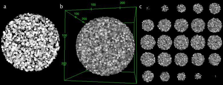 Shows the result of example 4a for the (a) two-dimensional, (b) three-dimensional and (c) four-dimensional case. The image series in (c) represents a movie of a three-dimensional rendering. The images of (b) and (c) were rendered using the ImageJ 3d Viewer.
import ij.ImageJ; import ij.ImagePlus; import java.util.Random; import net.imglib2.Point; import net.imglib2.RandomAccessibleInterval; import net.imglib2.algorithm.region.hypersphere.HyperSphere; import net.imglib2.algorithm.region.hypersphere.HyperSphereCursor; import net.imglib2.exception.ImgLibException; import net.imglib2.img.display.imagej.ImageJFunctions; import net.imglib2.img.imageplus.ImagePlusImg; import net.imglib2.img.imageplus.ImagePlusImgFactory; import net.imglib2.type.numeric.RealType; import net.imglib2.type.numeric.integer.UnsignedByteType; import net.imglib2.util.Util; /** * Draw a sphere full of little spheres */ public class Example4a { public Example4a() { // create an ImagePlusImg ImagePlusImg< UnsignedByteType, ? > img = new ImagePlusImgFactory<>( new UnsignedByteType() ).create( 256, 256, 256 ); // draw a small sphere for every pixel of a larger sphere drawSpheres( img, 0, 255 ); // display output and input try { ImagePlus imp = img.getImagePlus(); imp.show(); } catch ( ImgLibException e ) { System.out.println( "This ImagePlusImg does not hold a native " + "ImagePlus as container, either because the dimensionality is too " + "high or because the type is not supported." ); ImageJFunctions.show( img ); } } /** * Draws a sphere that contains lots of small spheres into the center of the interval * * @param randomAccessible - the image data to write to * @param minValue - the minimal intensity of one of the small spheres * @param maxValue - the maximal intensity of one of the small spheres */ public < T extends RealType< T > > void drawSpheres( final RandomAccessibleInterval< T > randomAccessible, final double minValue, final double maxValue ) { // the number of dimensions int numDimensions = randomAccessible.numDimensions(); // define the center and radius Point center = new Point( randomAccessible.numDimensions() ); long minSize = randomAccessible.dimension( 0 ); for ( int d = 0; d < numDimensions; ++d ) { long size = randomAccessible.dimension( d ); center.setPosition( size / 2 , d ); minSize = Math.min( minSize, size ); } // define the maximal radius of the small spheres int maxRadius = 5; // compute the radius of the large sphere so that we do not draw // outside of the defined interval long radiusLargeSphere = minSize / 2 - maxRadius - 1; // instantiate a random number generator Random rnd = new Random( System.currentTimeMillis() ); // define a hypersphere (n-dimensional sphere) HyperSphere< T > hyperSphere = new HyperSphere<>( randomAccessible, center, radiusLargeSphere ); // create a cursor on the hypersphere HyperSphereCursor< T > cursor = hyperSphere.cursor(); while ( cursor.hasNext() ) { cursor.fwd(); // the random radius of the current small hypersphere int radius = rnd.nextInt( maxRadius ) + 1; // instantiate a small hypersphere at the location of the current pixel // in the large hypersphere HyperSphere< T > smallSphere = new HyperSphere<>( randomAccessible, cursor, radius ); // define the random intensity for this small sphere double randomValue = rnd.nextDouble(); // take only every 4^dimension'th pixel by chance so that it is not too crowded if ( Math.round( randomValue * 100 ) % Util.pow( 4, numDimensions ) == 0 ) { // scale to right range randomValue = rnd.nextDouble() * ( maxValue - minValue ) + minValue; // set the value to all pixels in the small sphere if the intensity is // brighter than the existing one for ( final T value : smallSphere ) value.setReal( Math.max( randomValue, value.getRealDouble() ) ); } } } public static void main( String[] args ) { // open an ImageJ window new ImageJ(); // run the example new Example4a(); } }
Example 4b - Finding and displaying local minima
In this example we want to find all local minima in an image an display them as small spheres. To not capture too much of the noise in the image data, we first perform an in-place Gaussian smoothing with a sigma of 1, i.e. the data will be overwritten with the result. A complete documentation of the gauss package for ImgLib2 can be found here.
We display the results using a binary image. Note that the BitType only requires one bit per pixel and therefore is very memory efficient.
The generic method for minima detection has some more interesting properties.
The type of the source image data actually does not require to be of Type,
it simply needs something that is comparable. The LocalNeighborhood will
iterate n-dimensionally all pixels adjacent to a certain location, but skip the
central pixel (this corresponds to an both neighbors in 1d, an 8-neighborhood
in 2d, a 26-neighborhood in 3d, and so on …). This allows to efficiently
detect if a pixel is a local minima or maxima. Note that the Cursor that
performs the iteration can have special implementations for specific
dimensionalities to speed up the iteration. See below the example for a
specialized three-dimensional iteration:
Access plan for a 3d neighborhood, starting at the center position marked by (x). The initial position is, in this example, NOT part of iteration, which means the center pixel is not iterated. Note that every step except for the last one can be done with a very simple move command.
upper z plane (z-1) center z plane (z=0) lower z plane(z+1)
------------- ------------- -------------
| 2 | 1 | 8 | | 11| 10| 9 | | 20| 19| 18|
|------------ ------------- -------------
| 3 | 0 | 7 | | 12| x | 16| | 21| 25| 17|
|------------ ------------- -------------
| 4 | 5 | 6 | | 13| 14| 15| | 22| 23| 24|
------------- ------------- -------------
Please note as well that if one would increase the radius of the RectangleShape to more than 1 (without at the same time changing the View on source that creates an inset border of exactly this one pixel), this example would fail as we would try to write image data outside of the defined boundary. OutOfBoundsStrategies which define how to handle such cases is discussed in example 5.
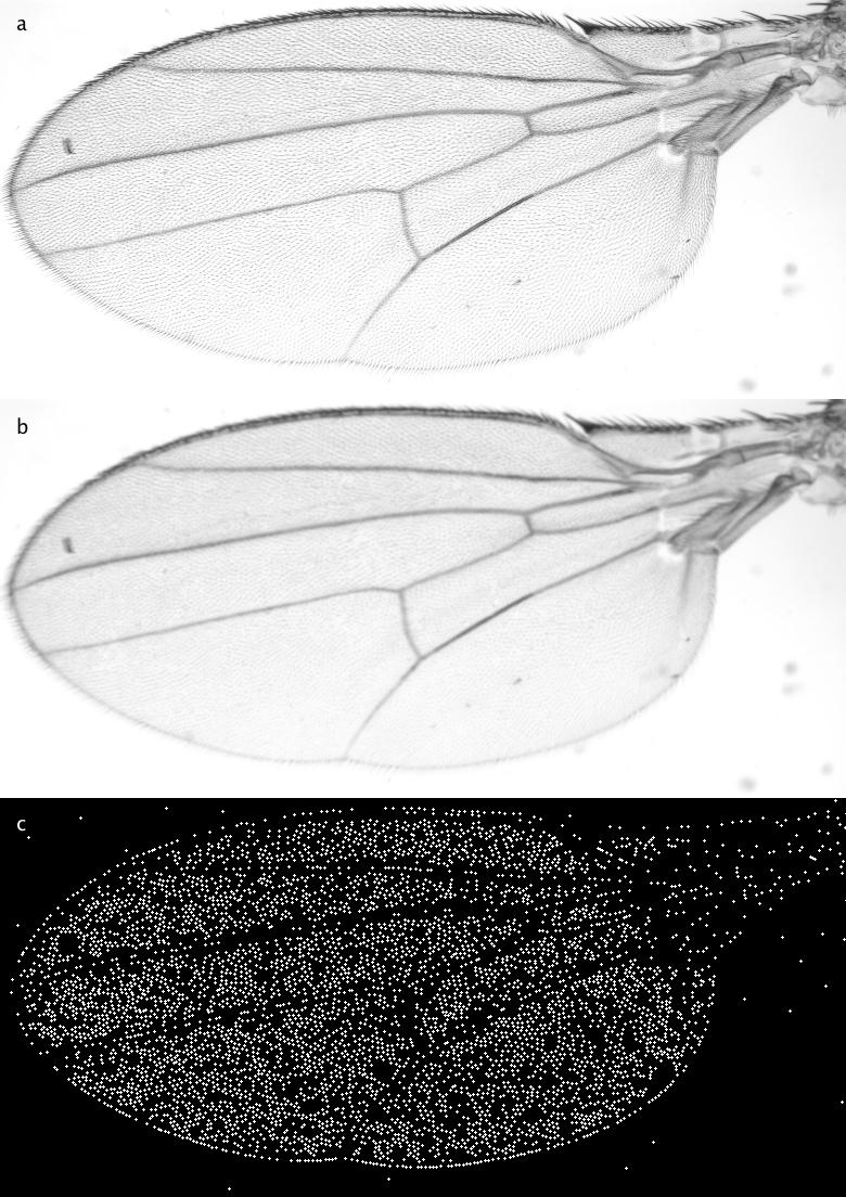 Shows the result of the detection of local minima after the Gaussian blurring. (a) depicts the input image, (b) the blurred version (sigma=1) and (c) all local mimina drawn as circles with radius 1.
import ij.ImageJ; import io.scif.img.IO; import io.scif.img.ImgIOException; import net.imglib2.Cursor; import net.imglib2.Interval; import net.imglib2.RandomAccessibleInterval; import net.imglib2.algorithm.gauss.Gauss; import net.imglib2.algorithm.neighborhood.Neighborhood; import net.imglib2.algorithm.neighborhood.RectangleShape; import net.imglib2.algorithm.region.hypersphere.HyperSphere; import net.imglib2.exception.IncompatibleTypeException; import net.imglib2.img.Img; import net.imglib2.img.ImgFactory; import net.imglib2.img.array.ArrayImgFactory; import net.imglib2.img.display.imagej.ImageJFunctions; import net.imglib2.type.NativeType; import net.imglib2.type.logic.BitType; import net.imglib2.type.numeric.RealType; import net.imglib2.util.Intervals; import net.imglib2.view.Views; /** * Here we use special cursors to find the local minima and * display them with spheres in another image */ public class Example4b { public < T extends RealType< T > & NativeType< T > > Example4b() throws ImgIOException { // open with SCIFIO Img< T > img = ( Img< T > ) IO.openImgs( "DrosophilaWing.tif" ).get( 0 ); // first we do a small in-place gaussian smoothing with a sigma of 1 Gauss.inDoubleInPlace( new double[]{ 1, 1 }, img ); // find local minima and paint them into another image as spheres Img< BitType > display = findAndDisplayLocalMinima( img, new ArrayImgFactory<>( new BitType() ) ); // display output and input ImageJFunctions.show( img ); ImageJFunctions.show( display ); } /** * Checks all pixels in the image if they are a local minima and * draws a circle into the output if they are * * @param source - the image data to work on * @param imageFactory - the factory for the output img * @return - an Img with circles on locations of a local minimum */ public static < T extends Comparable< T >, U extends RealType< U > > Img< U > findAndDisplayLocalMinima( RandomAccessibleInterval< T > source, ImgFactory< U > imageFactory ) { // Create a new image for the output Img< U > output = imageFactory.create( source ); // define an interval that is one pixel smaller on each side in each dimension, // so that the search in the 8-neighborhood (3x3x3...x3) never goes outside // of the defined interval Interval interval = Intervals.expand( source, -1 ); // create a view on the source with this interval source = Views.interval( source, interval ); // create a Cursor that iterates over the source and checks in a 8-neighborhood // if it is a minima final Cursor< T > center = Views.iterable( source ).cursor(); // instantiate a RectangleShape to access rectangular local neighborhoods // of radius 1 (that is 3x3x...x3 neighborhoods), skipping the center pixel // (this corresponds to an 8-neighborhood in 2d or 26-neighborhood in 3d, ...) final RectangleShape shape = new RectangleShape( 1, true ); // iterate over the set of neighborhoods in the image for ( final Neighborhood< T > localNeighborhood : shape.neighborhoods( source ) ) { // what is the value that we investigate? // (the center cursor runs over the image in the same iteration order as neighborhood) final T centerValue = center.next(); // keep this boolean true as long as no other value in the local neighborhood // is larger or equal boolean isMinimum = true; // check if all pixels in the local neighborhood that are smaller for ( final T value : localNeighborhood ) { // test if the center is smaller than the current pixel value if ( centerValue.compareTo( value ) >= 0 ) { isMinimum = false; break; } } if ( isMinimum ) { // draw a sphere of radius one in the new image HyperSphere< U > hyperSphere = new HyperSphere<>( output, center, 1 ); // set every value inside the sphere to 1 for ( U value : hyperSphere ) value.setOne(); } } return output; } public static void main( String[] args ) throws ImgIOException, IncompatibleTypeException { // open an ImageJ window new ImageJ(); // run the example new Example4b(); } }
Example 5 - Out of bounds
Many algorithms like convolutions require to access pixels outside of an Interval, i.e. also pixels outside of an image. In ImgLib2 this is handled using Views which convert a RandomAccessibleInterval into an infinite RandomAccessible using an OutOfBoundsStrategy. Those infinite RandomAccessibles are able to return pixel values at any arbitrary location.
Important: One should never access pixels outside of the defined Interval as it will in most cases result in unexpected behavior, depending on the kind of underlying RandomAccessible. If it is for example an Img, it will return wrong values or throw an exception.
Which OutOfBoundsStrategy to use depends on task you want to perform. For convolutions we suggest the mirror strategy as it introduces the least artifacts. When working on Fourier images, the periodic strategy applies best as it correctly mimics its spatial properties. Random Value strategies might be useful to avoid accidental correlations and constant value strategies are the most performant and might work well for simple operations or to avoid exceptions when accidental writing or reading outside of the Interval occurs.
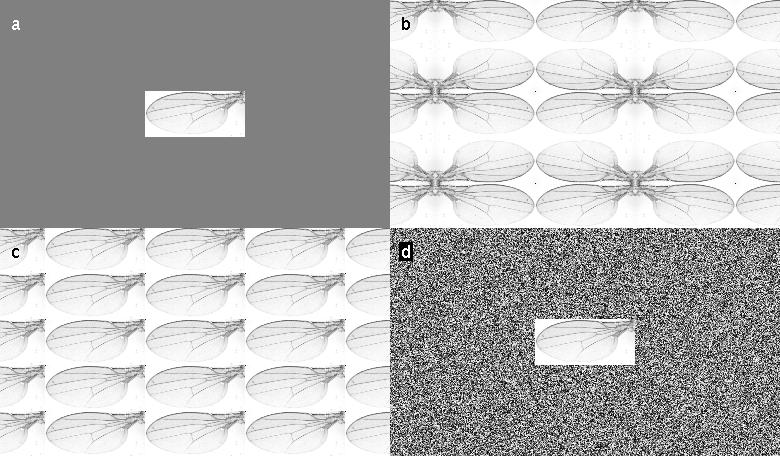 Illustrates the effect of various OutOfBoundsStrategies. (a) shows out of bounds with a constant value, (b) shows a mirroring strategy, (c) shows the periodic strategy, and (d) shows a strategy that uses random values.
import ij.ImageJ; import io.scif.img.IO; import io.scif.img.ImgIOException; import net.imglib2.FinalInterval; import net.imglib2.RandomAccessible; import net.imglib2.img.Img; import net.imglib2.img.display.imagej.ImageJFunctions; import net.imglib2.outofbounds.OutOfBoundsConstantValueFactory; import net.imglib2.type.numeric.real.FloatType; import net.imglib2.view.ExtendedRandomAccessibleInterval; import net.imglib2.view.Views; /** * Illustrate outside strategies * */ public class Example5 { public Example5() throws ImgIOException { // open with SCIFIO as a FloatType Img< FloatType > image = IO.openImgs( "DrosophilaWingSmall.tif", new FloatType() ).get( 0 ); // create an infinite view where all values outside of the Interval are 0 RandomAccessible< FloatType> infinite1 = Views.extendValue( image, new FloatType( 0 ) ); // create an infinite view where all values outside of the Interval are 128 RandomAccessible< FloatType> infinite2 = Views.extendValue( image, new FloatType( 128 ) ); // create an infinite view where all outside values are random in a range of 0-255 RandomAccessible< FloatType> infinite3 = Views.extendRandom( image, 0, 255 ); // create an infinite view where all values outside of the Interval are // the mirrored content, the mirror is the last pixel RandomAccessible< FloatType> infinite4 = Views.extendMirrorSingle( image ); // create an infinite view where all values outside of the Interval are // the mirrored content, the mirror is BEHIND the last pixel, // i.e. the first and last pixel are always duplicated RandomAccessible< FloatType> infinite5 = Views.extendMirrorDouble( image ); // all values outside of the Interval periodically repeat the image content // (like the Fourier space assumes) RandomAccessible< FloatType> infinite6 = Views.extendPeriodic( image ); // if you implemented your own strategy that you want to instantiate, it will look like this RandomAccessible< FloatType> infinite7 = new ExtendedRandomAccessibleInterval<>( image, new OutOfBoundsConstantValueFactory<>( new FloatType( 255 ) ) ); // visualize the outofbounds strategies // in order to visualize them, we have to define a new interval // on them which can be displayed long[] min = new long[ image.numDimensions() ]; long[] max = new long[ image.numDimensions() ]; for ( int d = 0; d < image.numDimensions(); ++d ) { // we add/subtract another 30 pixels here to illustrate // that it is really infinite and does not only work once min[ d ] = -image.dimension( d ) - 90 ; max[ d ] = image.dimension( d ) * 2 - 1 + 90; } // define the Interval on the infinite random accessibles FinalInterval interval = new FinalInterval( min, max ); // now define the interval on the infinite view and display ImageJFunctions.show( Views.interval( infinite1, interval ) ); ImageJFunctions.show( Views.interval( infinite2, interval ) ); ImageJFunctions.show( Views.interval( infinite3, interval ) ); ImageJFunctions.show( Views.interval( infinite4, interval ) ); ImageJFunctions.show( Views.interval( infinite5, interval ) ); ImageJFunctions.show( Views.interval( infinite6, interval ) ); ImageJFunctions.show( Views.interval( infinite7, interval ) ); } public static void main( String[] args ) throws ImgIOException { // open an ImageJ window new ImageJ(); // run the example new Example5(); } }
Example 6 - Basic built-in algorithms
ImgLib2 contains a growing number of built-in standard algorithms. In this section, we will show some of those, illustrate how to use them and give some examples of what it might be used for.
Typically algorithms provide static methods for simple calling, but they also have classes which you can instantiate yourself to have more options.
Important: Algorithms do not allow to work on a different dimensionality than the input data. You can achieve that by selecting hyperslices using Views (see Example 6a - version 4). In this way you can for example apply two-dimensional gaussians to each frame of a movie independently.
Example 6a - Gaussian convolution
The Gaussian convolution has its own wiki page. You can apply the Gaussian convolution with different sigmas in any dimension. It will work on any kind RandomAccessibleInterval. Below we show a examples of a simple gaussian convolution (variation 1), convolution using a different OutOfBoundsStrategy (variation 2), convolution of a part of an Interval (variation 3), and convolution of in a lower dimensionality than the image data (variation 4).
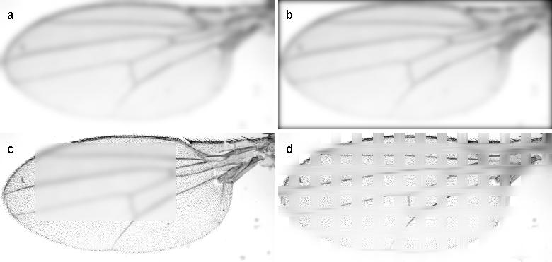 Shows the result of the four examples for Gaussian convolution. (a) shows a simple Gaussian convolution with sigma=8. (b) shows the same Gaussian convolution but using an OutOfBoundsConstantValue instead. (c) shows the result when convolving part of the image in-place. (d) shows the result when individually convolving 1-dimensional parts on the image.
Example 6a - Gaussian convolution (variation 1 - simple)
Here, we simply apply a Gaussian convolution with a sigma of 8. Note that it could be applied in-place as well when calling Gauss.inFloatInPlace( … ). The Gaussian convolution uses by default the OutOfBoundsMirrorStrategy.
import ij.ImageJ; import io.scif.img.IO; import io.scif.img.ImgIOException; import net.imglib2.algorithm.gauss.Gauss; import net.imglib2.img.Img; import net.imglib2.img.display.imagej.ImageJFunctions; import net.imglib2.type.numeric.real.FloatType; /** * Use of Gaussian Convolution on the Image * * @author Stephan Preibisch * @author Stephan Saalfeld */ public class Example6a1 { public Example6a1() throws ImgIOException { // open with SCIFIO as a FloatType Img< FloatType > image = IO.openImgs( "DrosophilaWing.tif", new FloatType() ).get( 0 ); // perform gaussian convolution with float precision double[] sigma = new double[ image.numDimensions() ]; for ( int d = 0; d < image.numDimensions(); ++d ) sigma[ d ] = 8; // convolve & display ImageJFunctions.show( Gauss.toFloat( sigma, image ) ); } public static void main( String[] args ) throws ImgIOException { // open an ImageJ window new ImageJ(); // run the example new Example6a1(); } }
Example 6a - Gaussian convolution (variation 2 - different OutOfBoundsStrategy)
Here we use an OutOfBoundsStrategyConstantValue instead. It results in continuously darker borders as the zero-values from outside of the image are used in the convolution. Note that the computation is done in-place here. However, we still need to provide an ImgFactory as the Gaussian convolution needs to create temporary image(s) - except for the one-dimensional case.
import ij.ImageJ; import io.scif.img.IO; import io.scif.img.ImgIOException; import net.imglib2.RandomAccessible; import net.imglib2.algorithm.gauss3.Gauss3; import net.imglib2.exception.IncompatibleTypeException; import net.imglib2.img.Img; import net.imglib2.img.display.imagej.ImageJFunctions; import net.imglib2.type.numeric.real.FloatType; import net.imglib2.view.Views; /** * Use of Gaussian Convolution on the Image * but convolve with a different outofboundsstrategy * * @author Stephan Preibisch * @author Stephan Saalfeld */ public class Example6a2 { public Example6a2() throws ImgIOException, IncompatibleTypeException { // open with SCIFIO as a FloatType Img< FloatType > image = IO.openImgs( "DrosophilaWing.tif", new FloatType() ).get( 0 ); // perform gaussian convolution with float precision double[] sigma = new double[ image.numDimensions() ]; for ( int d = 0; d < image.numDimensions(); ++d ) sigma[ d ] = 8; // first extend the image to infinity, zeropad RandomAccessible< FloatType > infiniteImg = Views.extendValue( image, new FloatType() ); // now we convolve the whole image manually in-place // note that is is basically the same as the call above, just called in a more generic way // // sigma .. the sigma // infiniteImg ... the RandomAccessible that is the source for the convolution // image ... defines the RandomAccessibleInterval that is the target of the convolution Gauss3.gauss( sigma, infiniteImg, image ); // show the in-place convolved image (note the different outofboundsstrategy at the edges) ImageJFunctions.show( image ); } public static void main( String[] args ) throws ImgIOException, IncompatibleTypeException { // open an ImageJ window new ImageJ(); // run the example new Example6a2(); } }
Example 6a - Gaussian convolution (variation 3 - only part of an Interval)
Here we only convolve part of an Interval, or in this case part of the Img. Note that for convolution he will actually use the real image values outside of the defined Interval. The OutOfBoundsStrategy is only necessary if the kernel is that large so that it will actually grep image values outside of the underlying Img.
Note: if you wanted, you could force him to use an OutOfBoundsStrategy directly outside of the Interval. For that you would have to create an RandomAccessibleInterval on the Img, extend it by an OutOfBoundsStrategy and give this as input to the Gaussian convolution.
import ij.ImageJ; import io.scif.img.IO; import io.scif.img.ImgIOException; import net.imglib2.FinalInterval; import net.imglib2.RandomAccessible; import net.imglib2.RandomAccessibleInterval; import net.imglib2.algorithm.gauss3.Gauss3; import net.imglib2.exception.IncompatibleTypeException; import net.imglib2.img.Img; import net.imglib2.img.display.imagej.ImageJFunctions; import net.imglib2.type.numeric.real.FloatType; import net.imglib2.util.Intervals; import net.imglib2.view.Views; /** * Use of Gaussian Convolution on the Image * but convolve just a part of the image * * @author Stephan Preibisch * @author Stephan Saalfeld */ public class Example6a3 { public Example6a3() throws ImgIOException, IncompatibleTypeException { // open with SCIFIO as a FloatType Img< FloatType > image = IO.openImgs( "DrosophilaWing.tif", new FloatType() ).get( 0 ); // perform gaussian convolution with float precision double sigma = 8; // we need to extend it nevertheless as the algorithm needs more pixels from around // the convolved area and we are not sure how much exactly (although we could compute // it with some effort from the sigma). // Here we let the Views framework take care of the details. The Gauss convolution // knows which area of the source image is required, and if the extension is not needed, // it will operate on the original image with no runtime overhead. RandomAccessible< FloatType> infiniteImg = Views.extendMirrorSingle( image ); // define the area of the image which we want to compute FinalInterval interval = Intervals.createMinMax( 100, 30, 500, 250 ); RandomAccessibleInterval< FloatType > region = Views.interval( image, interval ); // call the gauss, we convolve only a region and write it back to the exact same coordinates Gauss3.gauss( sigma, infiniteImg, region ); ImageJFunctions.show( image ); } public static void main( String[] args ) throws ImgIOException, IncompatibleTypeException { // open an ImageJ window new ImageJ(); // run the example new Example6a3(); } }
Example 6a - Gaussian convolution (variation 4 - with a lower dimensionality)
This example shows howto apply an algorithm to a lower dimensionality as the image data you are working on. Therefore we use Views to create HyperSlices which have n-1 dimensions. We simply apply the algorithm in-place on those Views which will automatically update the image data in the higher-dimensional data.
Specifically, we apply 1-dimensional Gaussian convolution in 30-pixel wide stripes using a sigma of 16. Note that whenever you request an HyperSlice for a certain dimension, you will get back a View that contains all dimensions but this one.
import ij.ImageJ; import io.scif.img.IO; import io.scif.img.ImgIOException; import net.imglib2.RandomAccessibleInterval; import net.imglib2.algorithm.gauss3.Gauss3; import net.imglib2.exception.IncompatibleTypeException; import net.imglib2.img.Img; import net.imglib2.img.display.imagej.ImageJFunctions; import net.imglib2.type.numeric.real.FloatType; import net.imglib2.view.Views; /** * Use of Gaussian Convolution on the Image * * @author Stephan Preibisch * @author Stephan Saalfeld */ public class Example6a4 { public Example6a4() throws ImgIOException, IncompatibleTypeException { // open with ImgOpener as a FloatType Img< FloatType > image = IO.openImgs( "DrosophilaWing.tif", new FloatType() ).get( 0 ); // perform all (n-1)-dimensional gaussian (in this case it means 1d) on // some of the row/columns double[] sigma = new double[ image.numDimensions() - 1 ]; for ( int d = 0; d < sigma.length; ++d ) sigma[ d ] = 16; // iterate over all dimensions, take always a hyperslice for ( int dim = 0; dim < image.numDimensions(); ++dim ) // iterate over all possible hyperslices for ( long pos = 0; pos < image.dimension( dim ); ++pos ) // convolve a subset of the 1-dimensional views if ( pos/30 % 2 == 1 ) { // get the n-1 dimensional "slice" RandomAccessibleInterval< FloatType > view = Views.hyperSlice( image, dim, pos ); // compute the gauss in-place on the view Gauss3.gauss( sigma, Views.extendMirrorSingle( view ), view ); } // show the result ImageJFunctions.show( image ); } public static void main( String[] args ) throws ImgIOException, IncompatibleTypeException { // open an ImageJ window new ImageJ(); // run the example new Example6a4(); } }
Example 6b - Convolution in Fourier space
In image processing it is sometimes necessary to convolve images with non-separable kernels. This can be efficiently done in Fourier space exploiting the convolution theorem. It states that a convolution in real-space corresponds to a multiplication in Fourier-space, as vice versa. Note that the computation time for such a convolution is independent of the size and shape of the kernel.
Note that it is useful to normalize the kernel prior to Fourier convolution so that the sum of all pixels is one. Otherwise, the resulting intensities will be increased.
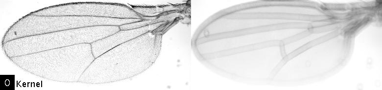 Shows the effect of the Fourier convolution. The left image was convolved with the kernel depicted in the lower left corner, the right panel shows the convolved image. Note that the computation speed does not depend on the size or the shape of the kernel.
Important: This source code is only GPLv2!
import ij.ImageJ; import io.scif.img.ImgIOException; import io.scif.img.ImgOpener; import net.imglib2.algorithm.fft2.FFTConvolution; import net.imglib2.exception.IncompatibleTypeException; import net.imglib2.img.Img; import net.imglib2.img.display.imagej.ImageJFunctions; import net.imglib2.type.numeric.RealType; import net.imglib2.type.numeric.real.FloatType; import net.imglib2.util.RealSum; /** * Perform a gaussian convolution using fourier convolution */ public class Example6b { public Example6b() throws ImgIOException, IncompatibleTypeException { // open with SCIFIO ImgOpener using an ArrayImgFactory final ImgOpener io = new ImgOpener(); final Img< FloatType > image = io.openImgs( "DrosophilaWing.tif", new FloatType() ).get( 0 ); final Img< FloatType > kernel = io.openImgs( "kernelRing.tif", new FloatType() ).get( 0 ); // normalize the kernel, otherwise we add energy to the image norm( kernel ); // display image & kernel ImageJFunctions.show( kernel ).setTitle( "kernel" ); ImageJFunctions.show( image ).setTitle( "drosophila wing"); // compute & show fourier convolution (in-place) new FFTConvolution<>( image, kernel ).convolve(); ImageJFunctions.show( image ) .setTitle( "convolution" ); } /** * Computes the sum of all pixels in an iterable using RealSum * * @param iterable - the image data * @return - the sum of values */ public static < T extends RealType< T > > double sumImage( final Iterable< T > iterable ) { final RealSum sum = new RealSum(); for ( final T type : iterable ) sum.add( type.getRealDouble() ); return sum.getSum(); } /** * Norms all image values so that their sum is 1 * * @param iterable - the image data */ public static void norm( final Iterable< FloatType > iterable ) { final double sum = sumImage( iterable ); for ( final FloatType type : iterable ) type.setReal( type.get() / sum ); } public static void main( final String[] args ) throws ImgIOException, IncompatibleTypeException { // open an ImageJ window new ImageJ(); // run the example new Example6b(); } }
Example 6c - Complex numbers and Fourier transforms
In this example we show how to work with complex numbers and Fourier transforms. We show how to determine the location of a template in an image exploiting the Fourier Shift Theorem. We therefore compute the Fast Fourier Transform of a template, invert it and convolve it in Fourier space with the original image.
Computing an FFT is straight forward. It does not offer a static method because the instance of the FFT is required to perform an inverse FFT. This is necessary because the input image needs to be extended to a size supported by the 1-d FFT method (edu_mines_jtk.jar). In order to restore the complete input image remembering those parameters is essential.
For the display of complex image data we provide Converters to display the gLog of the power-spectrum (default), phase-spectrum, real values, and imaginary values. It is, however, straight forward to implement you own Converters.
Note that for inverting the kernel we use methods defined for ComplexType, also the basic math operations add, mul, sub and div are implemented in complex math. The inverse FFT finally takes the instance of the FFT as a parameter from which it takes all required parameters for a correct inversion.
The final convolution of the inverse template with the image is performed using the FourierConvolution (see example 6b). Note that all possible locations of the template in the image have been tested. The peak in the result image clearly marks the location of the template, while the computation time for the whole operation takes less than a second.
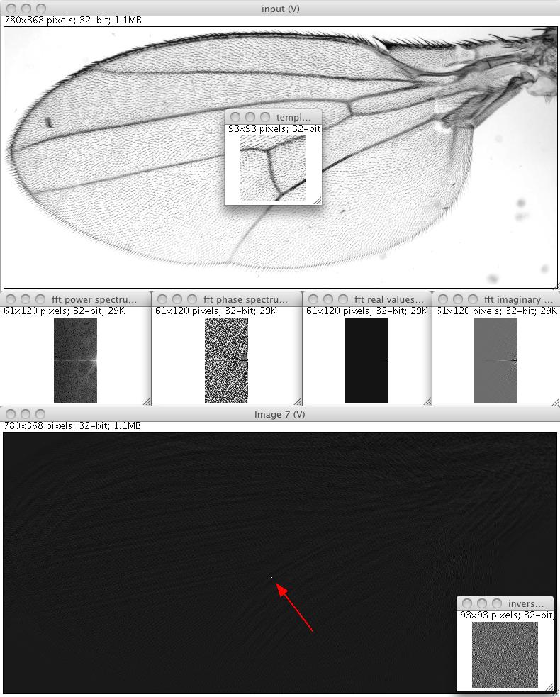 Shows the result and intermediate steps of the template matching using the Fourier space. In the upper panel you see the input image as well as the template that we use from matching. Below we show four different views of the Fast Fourier Transform of the template: the power spectrum, the phase spectrum, the real values, and the imaginary values. In the lower panel you see the result of the convolution of the inverse template with the image. The position where the template was located in the image is significantly visible. In the bottom right corner you see the inverse FFT of the inverse kernel.
Important: This source code is only GPLv2!
import io.scif.img.ImgIOException; import io.scif.img.ImgOpener; import net.imglib2.algorithm.fft.FourierConvolution; import net.imglib2.algorithm.fft.FourierTransform; import net.imglib2.algorithm.fft.InverseFourierTransform; import net.imglib2.converter.ComplexImaginaryFloatConverter; import net.imglib2.converter.ComplexPhaseFloatConverter; import net.imglib2.converter.ComplexRealFloatConverter; import net.imglib2.exception.IncompatibleTypeException; import net.imglib2.img.Img; import net.imglib2.img.display.imagej.ImageJFunctions; import net.imglib2.type.numeric.RealType; import net.imglib2.type.numeric.complex.ComplexFloatType; import net.imglib2.type.numeric.real.FloatType; import net.imglib2.util.RealSum; /** * Perform template matching by convolution in the Fourier domain * * @author Stephan Preibisch * @author Stephan Saalfeld */ public class Example6c { public Example6c() throws ImgIOException, IncompatibleTypeException { // open with SCIFIO ImgOpener as FloatTypes ImgOpener io = new ImgOpener(); final Img< FloatType > image = io.openImgs( "DrosophilaWing.tif", new FloatType() ).get( 0 ); final Img< FloatType > template = io.openImgs( "WingTemplate.tif", new FloatType() ).get( 0 ); // display image and template ImageJFunctions.show( image ).setTitle( "input" ); ImageJFunctions.show( template ).setTitle( "template" ); // compute fourier transform of the template final FourierTransform< FloatType, ComplexFloatType > fft = new FourierTransform<>(template, new ComplexFloatType() ); fft.process(); final Img< ComplexFloatType > templateFFT = fft.getResult(); // display fft (by default in generalized log power spectrum ImageJFunctions.show( templateFFT ).setTitle( "fft power spectrum" ); // display fft phase spectrum ImageJFunctions.show( templateFFT, new ComplexPhaseFloatConverter< ComplexFloatType >() ) .setTitle( "fft phase spectrum" ); // display fft real values ImageJFunctions.show( templateFFT, new ComplexRealFloatConverter< ComplexFloatType >() ) .setTitle( "fft real values" ); // display fft imaginary values ImageJFunctions.show( templateFFT, new ComplexImaginaryFloatConverter< ComplexFloatType >() ) .setTitle( "fft imaginary values" ); // complex invert the kernel final ComplexFloatType c = new ComplexFloatType(); for ( final ComplexFloatType t : templateFFT ) { c.set( t ); t.complexConjugate(); c.mul( t ); t.div( c ); } // compute inverse fourier transform of the template final InverseFourierTransform< FloatType, ComplexFloatType > ifft = new InverseFourierTransform<>( templateFFT, fft ); ifft.process(); final Img< FloatType > templateInverse = ifft.getResult(); // display the inverse template ImageJFunctions.show( templateInverse ).setTitle( "inverse template" ); // normalize the inverse template norm( templateInverse ); // compute fourier convolution of the inverse template and the image and display it ImageJFunctions.show( FourierConvolution.convolve( image, templateInverse ) ); } /** * Computes the sum of all pixels in an iterable using RealSum * * @param iterable - the image data * @return - the sum of values */ public static < T extends RealType< T > > double sumImage( final Iterable< T > iterable ) { final RealSum sum = new RealSum(); for ( final T type : iterable ) sum.add( type.getRealDouble() ); return sum.getSum(); } /** * Norms all image values so that their sum is 1 * * @param iterable - the image data */ public static void norm( final Iterable< FloatType > iterable ) { final double sum = sumImage( iterable ); for ( final FloatType type : iterable ) type.setReal( type.get() / sum ); } public static void main( final String[] args ) throws ImgIOException, IncompatibleTypeException { // open an ImageJ window new ImageJ(); // run the example new Example6c(); } }
Example 7 - Interpolation
Interpolation is a basic operation required in many image processing tasks. In the terminology of ImgLib2 it means to convert a RandomAccessible into a RealRandomAccessible which is able to create a RealRandomAccess. It can be positioned at real coordinates instead of only integer coordinates and a return a value for each real location. Currently, three interpolation schemes are available for ImgLib2:
- Nearest neighbor interpolation (also for available for any kind of data that can return a nearest neighbor like sparse datasets)
- Linear interpolation
- Lanczos interpolation
In the example we magnify a given real interval in the RealRandomAccessible which is based on the interpolation on an Img and compare the results of all three interpolation methods.
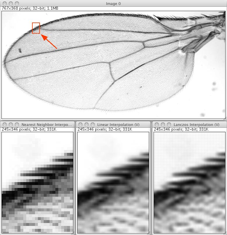 Shows the result for three different interpolators when magnifying a small part of the image by 10x. The nearest neighbor interpolation is computed fastest and is the most versatile as it requires no computation but just a lookout. The result is, however, very pixelated. The linear interpolation produces reasonable results and computes quite fast. The Lanczos interpolation shows visually most pleasing results but also introduces slight artifacts in the background.
import ij.ImageJ; import io.scif.img.IO; import io.scif.img.ImgIOException; import net.imglib2.Cursor; import net.imglib2.FinalRealInterval; import net.imglib2.RealInterval; import net.imglib2.RealRandomAccess; import net.imglib2.RealRandomAccessible; import net.imglib2.img.Img; import net.imglib2.img.ImgFactory; import net.imglib2.img.array.ArrayImgFactory; import net.imglib2.img.display.imagej.ImageJFunctions; import net.imglib2.interpolation.randomaccess.LanczosInterpolatorFactory; import net.imglib2.interpolation.randomaccess.NLinearInterpolatorFactory; import net.imglib2.interpolation.randomaccess.NearestNeighborInterpolatorFactory; import net.imglib2.type.Type; import net.imglib2.type.numeric.real.FloatType; import net.imglib2.view.Views; /** * Use three different interpolators to 10x magnify a small area */ public class Example7 { public Example7() throws ImgIOException { // open with SCIFIO Img< FloatType > img = IO.openImgs( "DrosophilaWing.tif", new FloatType() ).get( 0 ); ImageJFunctions.show( img ); // create an InterpolatorFactory RealRandomAccessible using nearst neighbor interpolation NearestNeighborInterpolatorFactory< FloatType > factory1 = new NearestNeighborInterpolatorFactory<>(); // create an InterpolatorFactory RealRandomAccessible using linear interpolation NLinearInterpolatorFactory< FloatType > factory2 = new NLinearInterpolatorFactory<>(); // create an InterpolatorFactory RealRandomAccessible using lanczos interpolation LanczosInterpolatorFactory< FloatType > factory3 = new LanczosInterpolatorFactory<>(); // create a RandomAccessible using the factory and views method // it is important to extend the image first, the interpolation scheme might // grep pixels outside of the boundaries even when locations inside are queried // as they integrate pixel information in a local neighborhood - the size of // this neighborhood depends on which interpolator is used RealRandomAccessible< FloatType > interpolant1 = Views.interpolate( Views.extendMirrorSingle( img ), factory1 ); RealRandomAccessible< FloatType > interpolant2 = Views.interpolate( Views.extendMirrorSingle( img ), factory2 ); RealRandomAccessible< FloatType > interpolant3 = Views.interpolate( Views.extendMirrorSingle( img ), factory3 ); // define the area in the interpolated image double[] min = new double[]{ 105.12, 40.43 }; double[] max = new double[]{ 129.56, 74.933 }; FinalRealInterval interval = new FinalRealInterval( min, max ); ImageJFunctions.show( magnify( interpolant1, interval, new ArrayImgFactory<>( new FloatType() ), 10 ) ).setTitle( "Nearest Neighbor Interpolation" ); ImageJFunctions.show( magnify( interpolant2, interval, new ArrayImgFactory<>( new FloatType() ), 10 ) ).setTitle( "Linear Interpolation" ); ImageJFunctions.show( magnify( interpolant3, interval, new ArrayImgFactory<>( new FloatType() ), 10 ) ).setTitle( "Lanczos Interpolation" ); } /** * Compute a magnified version of a given real interval * * @param source - the input data * @param interval - the real interval on the source that should be magnified * @param factory - the image factory for the output image * @param magnification - the ratio of magnification * @return - an Img that contains the magnified image content */ public static < T extends Type< T > > Img< T > magnify( RealRandomAccessible< T > source, RealInterval interval, ImgFactory< T > factory, double magnification ) { int numDimensions = interval.numDimensions(); // compute the number of pixels of the output and the size of the real interval long[] pixelSize = new long[ numDimensions ]; double[] intervalSize = new double[ numDimensions ]; for ( int d = 0; d < numDimensions; ++d ) { intervalSize[ d ] = interval.realMax( d ) - interval.realMin( d ); pixelSize[ d ] = Math.round( intervalSize[ d ] * magnification ) + 1; } // create the output image Img< T > output = factory.create( pixelSize ); // cursor to iterate over all pixels Cursor< T > cursor = output.localizingCursor(); // create a RealRandomAccess on the source (interpolator) RealRandomAccess< T > realRandomAccess = source.realRandomAccess(); // the temporary array to compute the position double[] tmp = new double[ numDimensions ]; // for all pixels of the output image while ( cursor.hasNext() ) { cursor.fwd(); // compute the appropriate location of the interpolator for ( int d = 0; d < numDimensions; ++d ) tmp[ d ] = cursor.getDoublePosition( d ) / output.realMax( d ) * intervalSize[ d ] + interval.realMin( d ); // set the position realRandomAccess.setPosition( tmp ); // set the new value cursor.get().set( realRandomAccess.get() ); } return output; } public static void main( String[] args ) throws ImgIOException { // open an ImageJ window new ImageJ(); // run the example new Example7(); } }
Example 8 - Working with sparse data
ImgLib2 supports sparsely sampled data, i.e. collections of locations together with their value. Such datasets typically implement the IterableRealInterval interface, which means they can be iterated and have real-valued locations in n-dimensional space. Currently ImgLib2 supports to store such collections either as list (RealPointSampleList) or KDTree. The RealPointSampleList can be iterated, whereas the KDTree additionally supports three efficient ways of searching for nearest neighboring points in the n-dimensional space (NearestNeighborSearch, KNearestNeighborSearch, and RadiusNeighborSearch).
In order to display sparse data ImgLib2 currently supports two interpolation schemes, the NearestNeighborInterpolation and the InverseDistanceWeightingInterpolation. They can compute a value for every location in space by returning either the value of the closest sample or an interpolated, distance-weighted value of the k nearest neighbors to the sampled location. The interpolation scheme therefore converts any IterableRealInterval into a RealRandomAccessible that can be displayed by wrapping it into a RandomAccessible and defining Interval using Views.
This is, however, not only useful for display. Note that you execute on such data any algorithm or method that is implemented for RealRandomAccessible or RandomAccessible, like Gaussian convolution in the first example. Note that none of these ever exists in memory, it is done completely virtual on just the sparse samples.
Example 8a - Create random sparse data, display and convolve it
In this example we create a certain number of random samples with random intensities inside a certain Interval. Using nearest neighbor interpolation we wrap it into a RealRandomAccessible, wrap it again into a RandomAccessible, define an Interval on it and display it. On the same virtual data we perform a Gaussian convolution and show it, too.
 On the left hand side it shows nearest-neighbor rendered random sparse data as created in example 8a. The right hand side shows the result of a Gaussian convolution, run directly on the virtual RandomAccessibleInterval.
import ij.ImageJ; import java.util.Random; import net.imglib2.FinalInterval; import net.imglib2.IterableRealInterval; import net.imglib2.KDTree; import net.imglib2.Point; import net.imglib2.RandomAccessible; import net.imglib2.RandomAccessibleInterval; import net.imglib2.RealInterval; import net.imglib2.RealPoint; import net.imglib2.RealPointSampleList; import net.imglib2.RealRandomAccessible; import net.imglib2.algorithm.gauss.Gauss; import net.imglib2.img.Img; import net.imglib2.img.array.ArrayImgFactory; import net.imglib2.img.display.imagej.ImageJFunctions; import net.imglib2.interpolation.neighborsearch.NearestNeighborSearchInterpolatorFactory; import net.imglib2.neighborsearch.NearestNeighborSearch; import net.imglib2.neighborsearch.NearestNeighborSearchOnKDTree; import net.imglib2.type.numeric.real.FloatType; import net.imglib2.view.Views; /** * Working with sparse data * * Create some random points with random values, display them and perform * a Gaussian convolution on the VIRTUAL data */ public class Example8a { public Example8a() { // the interval in which to create random points FinalInterval interval = new FinalInterval( new long[] { 375, 200 } ); // create an IterableRealInterval IterableRealInterval< FloatType > realInterval = createRandomPoints( interval, 250 ); // using nearest neighbor search we will be able to return a value an any position in space NearestNeighborSearch< FloatType > search = new NearestNeighborSearchOnKDTree<>( new KDTree<>( realInterval ) ); // make it into RealRandomAccessible using nearest neighbor search RealRandomAccessible< FloatType > realRandomAccessible = Views.interpolate( search, new NearestNeighborSearchInterpolatorFactory< FloatType >() ); // convert it into a RandomAccessible which can be displayed RandomAccessible< FloatType > randomAccessible = Views.raster( realRandomAccessible ); // set the initial interval as area to view RandomAccessibleInterval< FloatType > view = Views.interval( randomAccessible, interval ); // display the view ImageJFunctions.show( view ); // compute a gauss on it Img< FloatType > convolved = new ArrayImgFactory<>( new FloatType() ).create( interval ); Gauss.inFloat( new double[] { 3, 3 }, view, interval, convolved, new Point( view.numDimensions() ), convolved.factory() ); // display the view ImageJFunctions.show( convolved ); } /** * Create a number of n-dimensional random points in a certain interval * having a random intensity 0...1 * * @param interval - the interval in which points are created * @param numPoints - the amount of points * * @return a RealPointSampleList (which is an IterableRealInterval) */ public static RealPointSampleList< FloatType > createRandomPoints( RealInterval interval, int numPoints ) { // the number of dimensions int numDimensions = interval.numDimensions(); // a random number generator Random rnd = new Random( System.currentTimeMillis() ); // a list of Samples with coordinates RealPointSampleList< FloatType > elements = new RealPointSampleList<>( numDimensions ); for ( int i = 0; i < numPoints; ++i ) { RealPoint point = new RealPoint( numDimensions ); for ( int d = 0; d < numDimensions; ++d ) point.setPosition( rnd.nextDouble() * ( interval.realMax( d ) - interval.realMin( d ) ) + interval.realMin( d ), d ); // add a new element with a random intensity in the range 0...1 elements.add( point, new FloatType( rnd.nextFloat() ) ); } return elements; } public static void main( String[] args ) { // open an ImageJ window new ImageJ(); // run the example new Example8a(); } }
Example 8b - Randomly sample an existing image and display it
In this example we sample an existing image at random locations and render the result using a nearest neighbor interpolation as well as a distance-weighted average of the k nearest neighbors.
Shows the result of sparse sampling of an existing image using a varying number of random samples. The upper panel shows the rendering using nearest neighbor interpolation, the lower panel uses an interpolated, distance-weighted value of the k nearest neighbors relative to each sampled location (i.e. each pixel).
import ij.ImageJ; import io.scif.img.IO; import io.scif.img.ImgIOException; import java.util.Random; import net.imglib2.Interval; import net.imglib2.IterableRealInterval; import net.imglib2.KDTree; import net.imglib2.RandomAccessible; import net.imglib2.RandomAccessibleInterval; import net.imglib2.RealInterval; import net.imglib2.RealPoint; import net.imglib2.RealPointSampleList; import net.imglib2.RealRandomAccess; import net.imglib2.RealRandomAccessible; import net.imglib2.img.Img; import net.imglib2.img.display.imagej.ImageJFunctions; import net.imglib2.interpolation.neighborsearch.InverseDistanceWeightingInterpolatorFactory; import net.imglib2.interpolation.neighborsearch.NearestNeighborSearchInterpolatorFactory; import net.imglib2.interpolation.randomaccess.NLinearInterpolatorFactory; import net.imglib2.neighborsearch.KNearestNeighborSearch; import net.imglib2.neighborsearch.KNearestNeighborSearchOnKDTree; import net.imglib2.neighborsearch.NearestNeighborSearch; import net.imglib2.neighborsearch.NearestNeighborSearchOnKDTree; import net.imglib2.type.Type; import net.imglib2.type.numeric.RealType; import net.imglib2.type.numeric.real.FloatType; import net.imglib2.view.Views; /** * Working with sparse data, sample an existing image at random locations * and render it again using an increasing number of samples */ public class Example8b { public Example8b() throws ImgIOException { // open with SCIFIO using a FloatType Img< FloatType > img = IO.openImgs( "DrosophilaWingSmall.tif", new FloatType() ).get( 0 ); // show the image ImageJFunctions.show( img ); // use linear interpolation to convert the input into a RealRandomAccessible RealRandomAccessible< FloatType > realRandomAccessible = Views.interpolate( Views.extendMirrorSingle( img ), new NLinearInterpolatorFactory< FloatType >() ); // sample the image with an increasing number of random points and display the result for ( int numPoints = 2; numPoints <= 32768; numPoints = numPoints * 4 ) { // the result when we use nearest neighbor interpolation ImageJFunctions.show( randomSampling( realRandomAccessible, img, numPoints ), numPoints +" points (NN)" ); // the result when use a distance weighted interpolation of the 20 nearest neighbors ImageJFunctions.show( randomSamplingKNearest( realRandomAccessible, img, numPoints ), numPoints + " points (KNN)" ); } } /** * Sample randomly n points from the input and display the interpolated result * using nearest neighbors * * @param input - the input data * @param interval - the size of the input (where to collect random samples) * @param numPoints - how many points to sample * * @return - a RandomAccessibleInterval of the same size as the input, * rendered from the sparse data */ public < T extends Type< T > > RandomAccessibleInterval< T > randomSampling( RealRandomAccessible< T > input, Interval interval, int numPoints ) { // create an IterableRealInterval IterableRealInterval< T > realInterval = sampleRandomPoints( input, interval, numPoints ); // using nearest neighbor search we will be able to return a value an any position in space NearestNeighborSearch< T > search = new NearestNeighborSearchOnKDTree<>( new KDTree<>( realInterval ) ); // make it into RealRandomAccessible using nearest neighbor search RealRandomAccessible< T > realRandomAccessible = Views.interpolate( search, new NearestNeighborSearchInterpolatorFactory< T >() ); // convert it into a RandomAccessible which can be displayed RandomAccessible< T > randomAccessible = Views.raster( realRandomAccessible ); // set the initial interval as area to view return Views.interval( randomAccessible, interval ); } /** * Sample randomly n points from the input and display the interpolated result using * distance-weighted interpolation of 20 nearest neighbors * * @param input - the input data * @param interval - the size of the input (where to collect random samples) * @param numPoints - how many points to sample * * @return - a RandomAccessibleInterval of the same size as the input, * rendered from the sparse data */ public < T extends RealType< T > > RandomAccessibleInterval< T > randomSamplingKNearest( RealRandomAccessible< T > input, Interval interval, int numPoints ) { // create an IterableRealInterval IterableRealInterval< T > realInterval = sampleRandomPoints( input, interval, numPoints ); // using nearest neighbor search we will be able to return a value an any position in space KNearestNeighborSearch< T > search = new KNearestNeighborSearchOnKDTree< >( new KDTree<>( realInterval ), Math.min( 20, (int)realInterval.size() ) ); // make it into RealRandomAccessible using nearest neighbor search RealRandomAccessible< T > realRandomAccessible = Views.interpolate( search, new InverseDistanceWeightingInterpolatorFactory< T >() ); // convert it into a RandomAccessible which can be displayed RandomAccessible< T > randomAccessible = Views.raster( realRandomAccessible ); // set the initial interval as area to view return Views.interval( randomAccessible, interval ); } /** * Sample a number of n-dimensional random points in a certain interval having a * random intensity 0...1 * * @param interval - the interval in which points are created * @param numPoints - the amount of points * * @return a RealPointSampleList (which is an IterableRealInterval) */ public static < T extends Type< T > > RealPointSampleList< T > sampleRandomPoints( RealRandomAccessible< T > input, RealInterval interval, int numPoints ) { // the number of dimensions int numDimensions = interval.numDimensions(); // a random number generator Random rnd = new Random( 1332441549191l ); // a list of Samples with coordinates RealPointSampleList< T > elements = new RealPointSampleList<>( numDimensions ); // a random accessible in the image data to grep the right value RealRandomAccess< T > realRandomAccess = input.realRandomAccess(); for ( int i = 0; i < numPoints; ++i ) { RealPoint point = new RealPoint( numDimensions ); for ( int d = 0; d < numDimensions; ++d ) point.setPosition( rnd.nextDouble() * ( interval.realMax( d ) - interval.realMin( d ) ) + interval.realMin( d ), d ); realRandomAccess.setPosition( point ); // add a new element with a random intensity in the range 0...1 elements.add( point, realRandomAccess.get().copy() ); } return elements; } public static void main( String[] args ) throws ImgIOException { // open an ImageJ window new ImageJ(); // run the example new Example8b(); } }
