The content of this page has not been vetted since shifting away from MediaWiki. If you’d like to help, check out the how to help guide!
TrakEM2 is an ImageJ plugin for morphological data mining, three-dimensional modeling and image stitching, registration, editing and annotation.
See TrakEM2 snapshots for an overview.
Features
- Segmentation: manually draw areas across stacks, and sketch structures with balls and pipes. Skeletonize entire neuronal arborizations and represent synapses with relational connector objects.
- Measurements: volumes, surfaces, lengths, and also measurements via ImageJ ROIs.
- Image Registration: register floating image tiles to each other using SIFT and global optimization algorithms.
- 3D Visualization: interacting with the 3D Viewer plugin, TrakEM2 displays image volumes and 3D meshes of all kinds.
- Image Annotation: floating text labels.
- Semantic segmentation: order segmentations in tree hierarchies, whose template is exportable for reuse in other, comparable projects.
TrakEM2 interacts with the 3D Viewer for visualization of image volumes and 3D meshes.
TrakEM2 in Fiji
- Create new projects from “File - New - TrakEM2 (blank)”
- Open an existing project by dragging its .xml file onto the toolbar, or via “File - Open”.
Documentation
- How to
- Manual
- TrakEM2 tutorials with video tutorials.
- Examples of scripting in TrakEM2.
- Writing plugins for TrakEM2.
Running fiji for heavy-duty, memory-intensive, high-performance TrakEM2 tasks
The following configuration has been tested in a machine with 256 CPU cores and 1 TB of RAM, running Ubuntu 22.04, with the latest 1.8.0 JVM:
-Xms500g -Xmx500g -XX:+UseG1GC -verbose:gc -XX:+PrintGCDateStamps
Given that Fiji launches with the incremental garbage collector (via -Xincgc) instead of the concurrent one (via -XX:UseG1GC as above), you can’t just modify the ImageJ.cfg file like you would do to update the RAM usage (via -Xms500g -Xmx500g). Instead, do the following: generate a dry-run command in your terminal, pipe it into a text file, edit it to replace the -Xincgc for the G1 GC one, make the file executable, and launch it. This sed script can do that too:
$ ./ImageJ-linux64 --dry-run | sed 's/-Xincgc/-XX:+UseG1GC -verbose:gc -XX:+PrintGCDateStamps'/ >> launcher.sh
$ chmod +x launcher.sh
$ ./launcher.sh
What the JVM flags mean:
- -Xms500g : use an initial heap size of 500 Gb (i.e. start fiji with 500 Gb of RAM preallocated to it)
- -Xmx500g: use a maximum heap size of 500 Gb. Note it’s the same amount as the intial heap size, so that the heap cannot be resized.
- -XX:+UseG1GC : use the concurrent garbage collector. Clean up unused memory using parallel threads.
- -verbose:gc: optional, see when the garbage collector runs.
- -XX:+PrintGCDateStamps: see a record of when the GC is run.
With the above settings, we have succesfully registered tens of thousands of sections with millions of images in TrakEM2.
Preparing TrakEM2 for best performance
For fastest browsing through layers
Right-click on the canvas and choose “Display - Properties…”. Then make sure that:
- “snapshots mode” is set to “Disabled”, or at most to “Outlines”.
- “Prepaint” is not checked, so that it is disabled.
For importing large collections of images and editing them immediately afterwards
The goal is to avoid generating mipmaps multiple times, which may be very time consuming.
Right-click on the canvas and choose “Display - Properties…”. Then make sure that:
- “enable mipmaps” is not checked, so that it is disabled.
Beware that you will not be able to browse quickly through layers while importing, given that mipmaps will not be generated.
Now to correct the contrast, first re-enable mipmaps by going again to “Display - Properties…” and checking the “enable mipmaps” checkbox. Then you have two general (non-exclusive) options:
A. Use the built-in commands from the right-click menu, such as:
- “Adjust images - Enhance contrast layer-wise”
- “Adjust images - Set min and max layer-wise”
B. Create a preprocessor script and set it to all images. For example, a beanshell script to run CLAHE on each image. In the script, the patch and imp variables exist automatically, and represent the Patch instance and the ImagePlus instance that the Patch wraps, respectively.
import ij.IJ;
IJ.run(imp, "Enhance Local Contrast (CLAHE)", "blocksize=127"
   + " histogram=256 maximum=3 mask=*None* fast_(less_accurate)");
To set the script to all images, save the above to a file named “whatever.bsh” (notice the filename extension “.bsh”) and then right-click on the TrakEM2 canvas and choose “Script - Set preprocessor script layer-wise”, and choose the whole range of layers. This will set the script to every image of every layer, and trigger mipmap regeneration for every image. When TrakEM2 loads the image, the script will run on the image before TrakEM2 ever sees its contents.
The preprocessor script gives you maximum power: do whatever you want with the image. For example, normalize the image relative to a known good mean and standard deviation for your data set.
For regenerating mipmaps the fastest possible
The default generation of mipmaps is done with are averaging, and is pretty fast. Still, you may want to consider parallelizing it: go to “Project - Properties…”, and set the mipmap threads to the number of cores in your machine, for example 12.
Stop reading if you are satisfied with the default quality of scaled images in TrakEM2.
If you choose to generate mipmaps using Gaussians, go to “Project - Properties…”, and set the mipmaps mode to “Gaussian”. Then, you must take care of the following:
In TrakEM2 0.9a and later, the mipmaps machinery can use a multi-threaded Gaussian implementation now present in the latest ImageJ. This means that now there are two sets of threads:
- The set of threads, where each thread regenerates the mipmap pyramid of a single image.
- The set of threads that performs Gaussian blurring for downsampling, for each scaling iteration in the generation of the mipmap pyramid.
If your machine has 12 cores, the default settings will use 1 thread for mipmaps and 12 threads for gaussian blurring. This may not fit your data properties: you may end up waiting long times for mipmap generation if your images are small.
Two strategies are possible for accelerating Gaussian-based generation of mipmaps:
- Strategy A: your data consists of large images (over 4000x4000). Right-click on the TrakEM2 display and choose “Project - Properties…”, and set the mipmap threads to 1 (the default). Now, mipmaps will be regenerated for one single image at a time, using 12 threads (given 12 cores) for computing the Gaussians.
- Strategy B: your data consists of small images (smaller than 4000x4000). Go to the Fiji window and select “Edit - Options - Memory & Threads…”, and set the number of threads to 1. Then, go to “Project - Properties…”, and set the mipmap threads to 12. Now, mipmaps will be regenerated for 12 images at a time (given 12 cores), using a single thread for each to compute the Gaussians.
Use strategy A as well if your computer has little RAM, or if access to the images is slow and contentious (such as if the data lives in a USB hard drive). That’s why the default is one single thread for generating mipmaps.
If you change the method for generating mipmaps to a non-Gaussian method, the above situation does not occur. Set the number of threads for regenerating mipmaps to the number of cores, or less if your computer doesn’t have much RAM.
Faster XML loading and less memory consumption with larger quadtree buckets
Besides choosing an appropriate mipmap generation strategy for large images, make sure that you set as well the bucket size appropriately.
What is a bucket in TrakEM2: each layer (each section) has an internal Quadtree to be able to find an object (e.g. an image) under the mouse, or to be able to quickly find images that overlap with other images. In other words, to be able to perform fast spatial queries such as finding the list of all images that intersect a given rectangle.
If the bucket size is small (the default is 4096 pixels on the side, and a bucket is then a square of 4096x4096 pixels, which could be considered quite small), then in combination with a very large canvas size there will be way too many buckets generated. Will take a lot of time and also consume a lot of memory.
If your sections only have about 100 images each, and images are somewhat large (say, each has dimensions of 8096x8096 pixels), then set the bucket size to a much larger value than the default, for example to 100000. Effectively there will be only one bucket.
Small buckets make sense when there are many small objects in a layer or many small zdisplayable objects. In that situation, such as a single image per layer, but many smaller Ball or Pipe or AreaList objects on it, then go for the default bucket size (4096) or smaller. Otherwise, go for big or even very big, effectively removing the buckets functionality and reducing to list search, which is just fine for small lists of images like about 100.
When registering/aligning a collection of 400,000 images spread over 5,000 sections, it makes sense to make the buckets large (like 40960, 10x the default, or even larger than that).
Setting the bucket size to a large value will reduce XML loading time a lot.
To set the bucket size, right-click and choose “Display - Properties …” and write in the bucket size value.
How much RAM should I allocate to the JVM for Fiji to run TrakEM2?
Use a computer that follows this rule of thumb: take the largest single 2D image in your dataset, then multiply its size by 10, and make sure that every core of your CPU has at least that much RAM available to it.
For example, for a 4096x4096 16-bit image you will need at least 335 Mb per core, so at least 5.4 Gb of RAM for 16 cores. 8 Gb would likely work better. 32 Gb will be a pleasure to use.
As for a graphics card buy the largest you can afford, both in computing power and in internal memory.
Examples
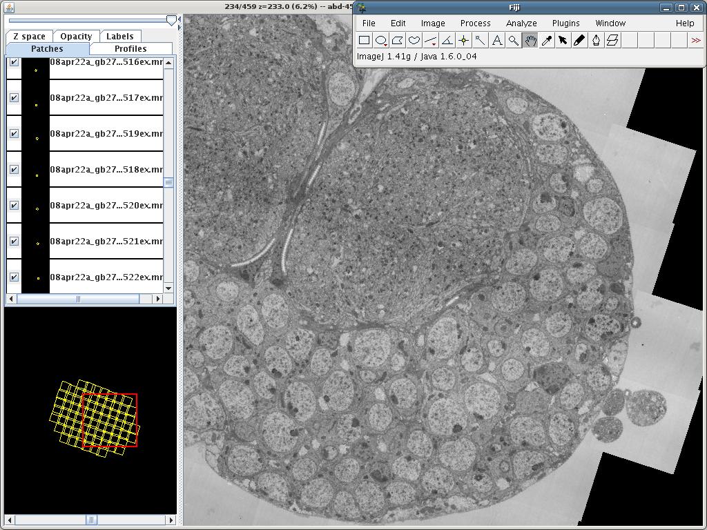 TrakEM2: 359 montages of 13x13 tiles of 2048x2048 pixels each.
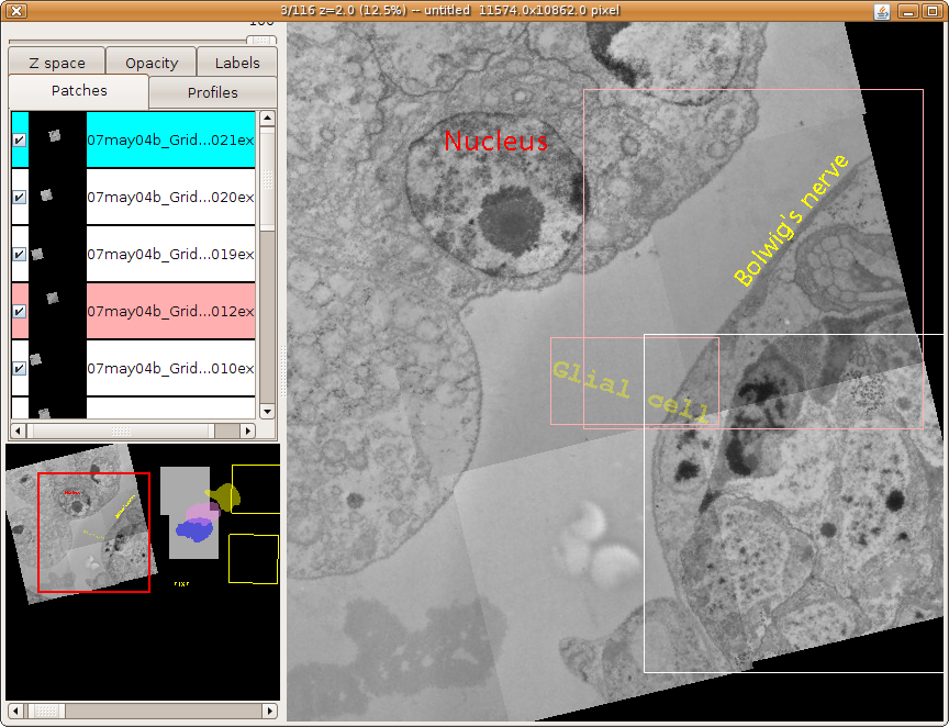 fig:TrakEM2 Display showing 9 images in a layer, where 2 images and one floating text label (set to 30% transparency) are selected (pink and white frames; white is the active one – note the corresponding pink and blue coloration of the object panels on the left). The Navigator (bottom left) paints a red frame to indicate the area currently displayed in the canvas (right).
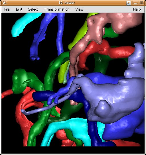 3D Viewer: hardware-accelerated 3D visualization of image stacks as volumes, orthoslices and meshes. Above, secondary lineages of Drosophila third instar larval brain segmented in TrakEM2.
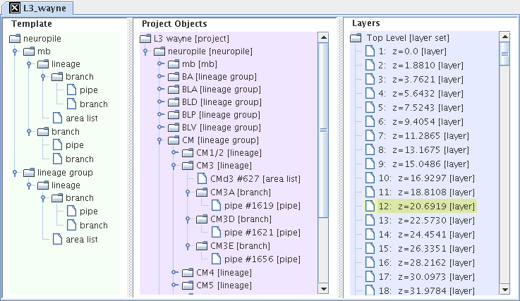 The three TrakEM2 trees, as an interface for editing and visualizing the three internal TrakEM2 data structures.
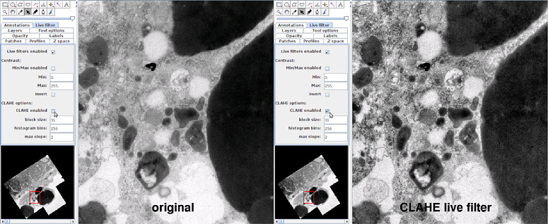 Effect of the CLAHE live filter in TrakEM2. Data with high dynamic range is displayed with perceptually boosted local contrast. CLAHE parameters are relative to display pixels and, therefore, will not result in an effective bandpass when zooming out largely on statically pre-processed images.
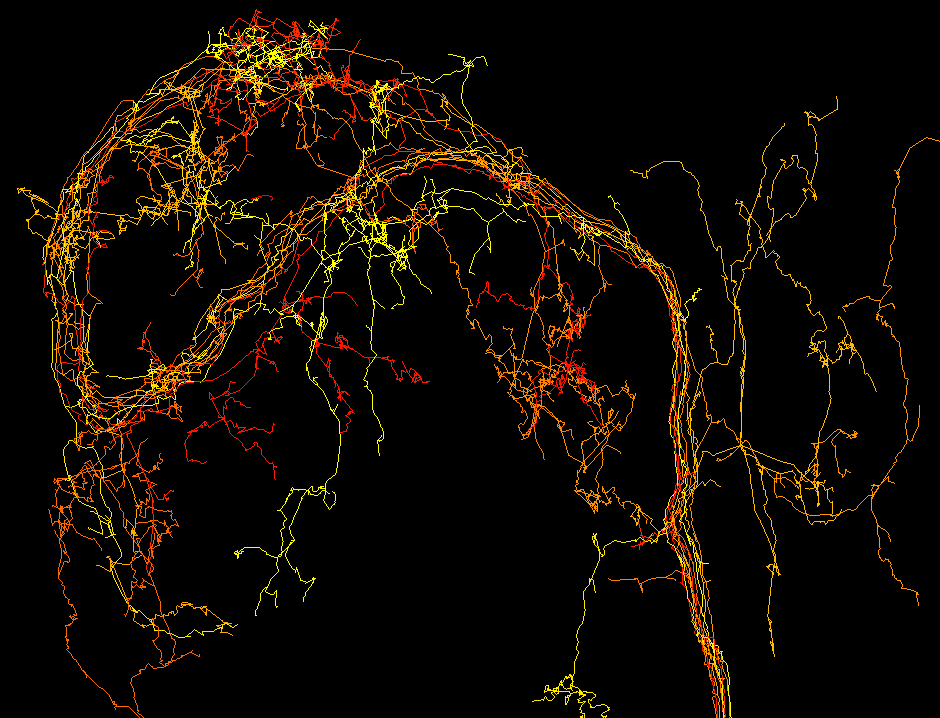 Neuronal arbors reconstructed with TrakEM2 using the treeline segmentation type.
 Neuronal arbors from serial section electron microscopy reconstructed with TrakEM2 using the manually segmentated data set.
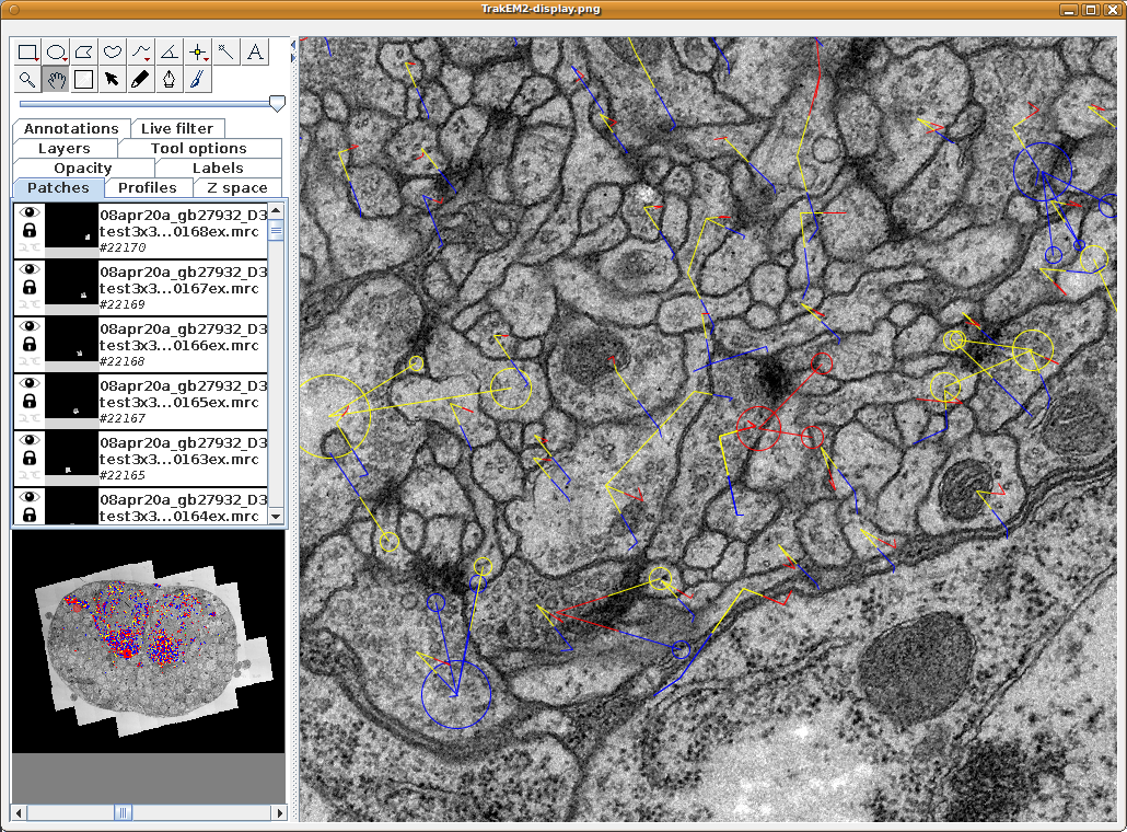 TrakEM2 showing one section of a serial section transmission electron microscopy (ssTEM) data set, with numerous neuronal arbors reconstructed using treelines and connectors (for synapses).
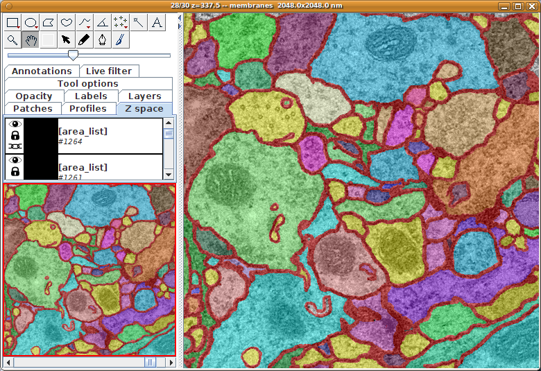
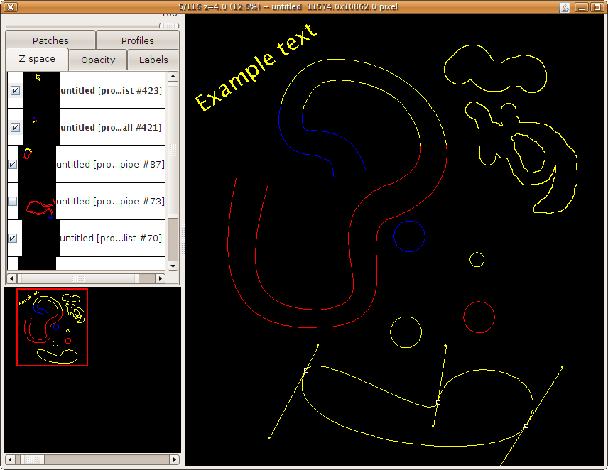 Example TrakEM2 segmentations, including Ball, Pipe, Profile, AreaList and floating text labels.